To convert a given Boolean value to a string in Python, use the str(boolean) function and pass the Boolean value into it. This converts Boolean True to string "True" and Boolean False to string "False".
Here’s a minimal example:
>>> str(True) 'True'
>>> str(False) 'False'
Python Boolean Type is Integer
Booleans are represented by integers in Python, i.e., bool is a subclass of int. Boolean value True is represented with integer 1. And Boolean value False is represented with integer 0.
Here’s a minimal example:
>>> True == 1
True
>>> False == 0
True
Convert True to ‘1’ and False to ‘0’
To convert a Boolean value to a string '1' or '0', use the expression str(int(boolean)). For instance, str(int(True)) returns '1' and str(int(False)) returns '0'. This is because of Python’s use of integers to represent Boolean values.
Here’s a minimal example:
>>> str(int(True)) '1'
>>> str(int(False)) '0'
Convert List of Boolean to List of Strings
To convert a Boolean to a string list, use the list comprehension expression [str(x) for x in my_bools] assuming the Boolean list is stored in variable my_bools. This converts each Boolean x to a string using the built-in str() function and repeats it for all x in the Boolean list.
Here’s a simple example:
my_bools = [True, True, False, False, True]
my_strings = [str(x) for x in my_bools]
print(my_strings)
# ['True', 'True', 'False', 'False', 'True']
Convert String Back to Boolean
What if you want to convert the string representation 'True' and 'False' (or: '1' and '0') back to the Boolean representation True and False?
You can convert a string value s to a Boolean value using the Python function bool(s).
For example, bool('True') and bool('1') return True.
However, bool('False') and bool('0') return False as well which may come unexpected to you.
This is because all Python objects are “truthy”, i.e., they have an associated Boolean value. As a rule of thumb: empty values return Boolean True and non-empty values return Boolean False. So, only bool('') on the empty string '' returns False. All other strings return True!
Easy – first pass the string into the eval() function and then pass the result into the bool() function. In other words, the expression bool(eval(my_string)) converts a string to a Boolean mapping 'True' and '1' to Boolean True and 'False' and '0' to Boolean False.
Finally – this behavior is as expected by many coders just starting out.
A Time Series is essentially a tabular data with the special feature of having a time index. The common forecast taks is ‘knowing the past (and sometimes the present), predict the future’. This task, taken as a principle, reveals itself in several ways: in how to interpret your problem, in feature engineering and in which forecast strategy to take.
This is the second article in our series. In the first article we discussed how to create features out of a time series using lags and trends. Today we follow the opposite direction by highlighting trends as something you want directly deducted from your model.
Reason is, Machine Learning models work in different ways. Some are good with subtractions, others are not.
For example, for any feature you include in a Linear Regression, the model will automatically detect whether to deduce it from the actual data or not. A Tree Regressor (and its variants) will not behave in the same way and usually will ignore a trend in the data.
Therefore, whenever using the latter type of models, one usually calls for a hybrid model, meaning, we use a Linear(ish) first model to detect global periodic patterns and then apply a second Machine Learning model to infer more sophisticated behavior.
The hybrid model part of this article is heavily based on Kaggle’s Time Series Crash Course, however, we intend to automate the process and discuss more in-depth the DeterministicProcess class.
DeterministicProcess aims at creating features to be used in a Regression model to determine trend and periodicity. It takes your DatetimeIndex and a few other parameters and returns a DataFrame full of features for your ML model.
A usual instance of the class will read like the one below. We use the sentic_mean column to illustrate.
from statsmodels.tsa.deterministic import DeterministicProcess y = dataset['sentic_mean'].copy() dp = DeterministicProcess(
index=y.index, constant=True, order=2
) X = dp.in_sample() X
We can use X and y as features and target to train a LinearRegression model. In this way, the LinearRegression will learn whatever characteristics from y can be inferred (in our case) solely out of:
the number of elapsed time intervals (trend column);
the last number squared (trend_squared); and
a bias term (const).
Check out the result:
from sklearn.linear_model import LinearRegression model = LinearRegression().fit(X,y) predictions = pd.DataFrame( model.predict(X), index=X.index, columns=['Deterministic Curve']
)
Even the quadratic term seems ignorable here. The DeterministicProcess class also helps us with future predictions since it carries a method that provides the appropriate future form of the chosen features.
Specifically, the out_of_sample method of dp takes the number of time intervals we want to predict as input and generates the needed features for you.
Although the order-three polynomial fits the data better, use discretion in deciding whether the sentiment count will decrease so drastically in the next 60 days or not. Usually, trust short-time predictions rather than long ones.
DeterministicProcess accepts other parameters, making it a very interesting tool. Find a description of the almost full list below.
dp = DeterministicProcess( index, # the DatetimeIndex of your data period: int or None, # in case the data shows some periodicity, include the size of the periodic cycle here: 7 would mean 7 days in our case constant: bool, # includes a constant feature in the returned DataFrame, i.e., a feature with the same value for everyone. It returns the equivalent of a bias term in Linear Regression order: int, # order of the polynomial that you think better approximates your trend: the simplest the better seasonal: bool, # make it True if you think the data has some periodicity. If you make it True and do not specify the period, the dp will try to infer the period out of the index additional_terms: tuple of statsmodel's DeterministicTerms, # we come back to this next drop: bool # drops resulting features which are collinear to others. If you will use a linear model, make it True
)
Seasonality
As a hardened Mathematician, seasonality is my favorite part because it deals with Fourier analysis (and wave functions are just… cool!):
Do you remember your first ML course when you heard Linear Regression can fit arbitrary functions, not only lines? So, why not a wave function? We just did it for polynomials and didn’t even feel like it
In general, for any expression f which is a function of a feature or of your DatetimeIndex, you can create a feature column whose ith row is the value of f corresponding to the ith index.
Then linear regression finds the constant coefficient multiplying f that best fits your data. Again, this procedure works in general, not only with Datetime indexes – the trend_squared term above is an example of it.
For seasonality, we use a second statsmodel‘s amazing class: CalendarFourier. It is another statsmodel‘s DeterministicTerm class (i.e., with the in_sample and out_of_sample methods) and instantiates with two parameters, 'frequency' and 'order'.
As a 'frequency', the class expects a string such as ‘D’, ‘W’, ‘M’ for day, week or month, respectively, or any of the quite comprehensive Pandas Datetime offset aliases.
The 'order' is the Fourier expansion order which should be understood as the number of waves you are expecting in your chosen frequency (count the number of ups and downs – one wave would be understood as one up and one down)
CalendarFourier integrates swiftly with DeterministicProcess by including an instance of it in the list of additional_terms.
If we take seasonal=True inside DeterministicProcess, we get a crispier line:
Including ax.set_xlim(('2022-08-01', '2022-10-01')) before plt.show() zooms the graph in:
Although I suggest using the seasonal=True parameter with care, it does find interesting patterns (with huge RMSE error, though).
For instance, look at this BTC percentage change zoomed chart:
Here period is set to 30 and seasonal=True. I also manually rescaled the predictions to be better visible in the graphic. Although the predictions are far away from truth, thinking as a trader, isn’t it impressive how many peaks and hills it gets right? At least for this zoomed month…
To maintain the workflow promise, I prepared a code that does everything so far in one shot:
def deseasonalize(df: pd.Series, season_freq='A', fourier_order=0, constant=True, dp_order=1, dp_drop=True, model=LinearRegression(), fourier=None, dp=None, **DeterministicProcesskwargs)->(pd.Series, plt.Axes, pd.DataFrame): """ Returns a deseasonalized and detrended df, a seasonal plot, and the fitted DeterministicProcess instance. """ if fourier is None: fourier = CalendarFourier(freq=season_freq, order=fourier_order) if dp is None: dp = DeterministicProcess( index=df.index, constant=True, order=dp_order, additional_terms=[fourier], drop=dp_drop, **DeterministicProcesskwargs ) X = dp.in_sample() model = LinearRegression().fit(X, df) y_pred = pd.Series( model.predict(X), index=X.index, name=df.name+'_pred' ) ax = plt.subplot() y.plot(ax=ax, legend=True) predictions.plot(ax=ax) y_pred.columns = df.name y_deseason = df - y_pred y_deseason.name = df.name +'_deseasoned' return y_deseason, ax, dp The sentic_mean analyses get reduced to: y_deseason, ax, dp= deseasonalize(y, season_freq='A', fourier_order=2, constant=True, dp_order=2, dp_drop=True, model=LinearRegression() )
Cycles and Hybrid Models
Let us move on to a complete Machine Learning prediction. We use XGBRegressor and compare its performance among three instances:
Predict sentic_mean directly using lags;
Same prediction adding the seasonal/trending with a DeterministicProcess;
A hybrid model, using LinearRegression to infer and remove seasons/trends, and then apply a XGBRegressor.
The first part will be the bulkier since the other two follow from simple modifications in the resulting code.
Preparing the data
Before any analysis, we split the data in train and test sets. Since we are dealing with time series, this means we set the ‘present date’ as a point in the past and try to predict its respective ‘future’. Here we pick 22 days in the past.
s = dataset['sentic_mean'] s_train = s[:'2022-09-01']
We made this first split in order to not leak data while doing any analysis.
Next, we prepare target and feature sets. Recall our SentiCrypto’s data was set to be available everyday at 8AM. Imagine we are doing the prediction by 9AM.
In this case, anything until the present data (the ‘lag_0‘) can be used as features, and our target is s_train‘s first lead (which we define as a -1 lag). To choose other lags as features, we examine theirs statsmodel’s partial auto-correlation plot:
from statsmodels.graphics.tsaplots import plot_pacf plot_pacf(s_train, lags=20)
We use the first four for sentic_mean and the first seven + the 11th for sentic_count (you can easily test different combinations with the code below.)
Now we finish choosing features, we go back to the full series for engineering. We apply to s_maen and s_count the make_lags function we defined in the last article (which we transcribe here for convenience).
def make_lags(df, n_lags=1, lead_time=1): """ Compute lags of a pandas.Series from lead_time to lead_time + n_lags. Alternatively, a list can be passed as n_lags. Returns a pd.DataFrame whose ith column is either the i+lead_time lag or the ith element of n_lags. """ if isinstance(n_lags,int): lag_list = list(range(lead_time, n_lags+lead_time)) else: lag_list = n_lags lags ={ f'{df.name}_lag_{i}': df.shift(i) for i in lag_list } return pd.concat(lags,axis=1) X = make_lags(s, [0,1,2,3,4]) y = make_lags(s, [-1]) display(X)
y
Now a train-test split with sklearn is convenient (Notice the shuffle=False parameter, that is key for time series):
from sklearn.model_selection import train_test_split X_train, X_test, y_train, y_test = train_test_split(X, y, test_size=22, shuffle=False) X_train
(Observe that the final date is set correctly, in accordance with our analysis’ split.)
You can reduce overfitness by reducing the number of estimators, but the R2 test score maintains negative.
We can replicate the process for sentic_count (or whatever you want). Below is a function to automate it.
from xgboost import XGBRegressor
from sklearn.model_selection import train_test_split
from sklearn.metrics import r2_score
from statsmodels.tsa.stattools import pacf def apply_univariate_prediction(series, test_size, to_predict=1, nlags=20, minimal_pacf=0.1, model=XGBRegressor(n_estimators=50)): ''' Starting from series, breaks it in train and test subsets; chooses which lags to use based on pacf > minimal_pacf; and applies the given sklearn-type model. Returns the resulting features and targets and the trained model. It plots the graph of the training and prediction, together with their r2_score. ''' s = series.iloc[:-test_size] if isinstance(to_predict,int): to_predict = [to_predict] from statsmodels.tsa.stattools import pacf s_pacf = pd.Series(pacf(s, nlags=nlags)) column_list = s_pacf[s_pacf>minimal_pacf].index X = make_lags(series, n_lags=column_list).dropna() y = make_lags(series,n_lags=[-x for x in to_predict]).loc[X.index] X_train, X_test, y_train, y_test = train_test_split(X, y, test_size=test_size, shuffle=False) model.fit(X_train,y_train) predictions_train = pd.DataFrame( model.predict(X_train), index=X_train.index, columns=['Train Predictions'] ) predictions_test = pd.DataFrame( model.predict(X_test), index=X_test.index, columns=['Test Predictions'] ) fig, (ax1,ax2) = plt.subplots(1,2, figsize=(14,5), sharey=True) y_train.plot(ax=ax1, legend=True) predictions_train.plot(ax=ax1) ax1.set_title('Train Predictions') y_test.plot(ax=ax2, legend=True) predictions_test.plot(ax=ax2) ax2.set_title('Test Predictions') plt.show() print(f'R2 train score: {r2_score(y_train[:-1],predictions_train[:-1])}') print(f'R2 test score: {r2_score(y_test[:-1],predictions_test[:-1])}') return X, y, model apply_univariate_prediction(dataset['sentic_count'],22)
Since the features created by DeterministicProcess are only time-dependent, we can add them harmlessly to the feature DataFrame we automated get from our univariate predictions.
The predictions, though, are still univariate. We use the deseasonalize function to obtain the season features. The data preparation is as follows:
s = dataset['sentic_mean'] X, y, _ = apply_univariate_prediction(s,22); s_deseason, _, dp = deseasonalize(s, season_freq='A', fourier_order=2, constant=True, dp_order=2, dp_drop=True, model=LinearRegression() );
X_f = dp.in_sample().shift(-1) X = pd.concat([X,X_f], axis=1, join='inner').dropna()
With a bit of copy and paste, we arrive at:
And we actually perform way worse!
Deseasonalizing
Nevertheless, the right-hand graphic illustrates the inability of grasping trends. Our last shot is a hybrid model.
Here we follow three steps:
We use the LinearRegression to capture the seasons and trends, rendering the series y_s. Then we acquire a deseasonalized target y_ds = y-y_s;
Train an XGBRegressor on y_ds and the lagged features, resulting in deseasonalized predictions y_pred;
Finally, we incorporate y_s back to y_pred to compare the final result.
Although Bitcoin-related data are hard to predict, there was a huge improvement on the r2_score (finally something positive!). We define the used function below.
Instead of going through every detail, we will also automate this code. In order to get the code running smoothly, we revisit the deseasonalize and the apply_univariate_prediction functions in order to remove the plotting part of them.
The final function only plots graphs and returns nothing. It intends to give you a baseline for a hybrid model score. Change the function at will to make it return whatever you need.
def get_season(series: pd.Series, test_size, season_freq='A', fourier_order=0, constant=True, dp_order=1, dp_drop=True, model1=LinearRegression(), fourier=None, is_seasonal=False, season_period=None, dp=None): """ Decompose series in a deseasonalized and a seasonal part. The parameters are relative to the fourier and DeterministicProcess used. Returns y_ds and y_s. """ se = series.iloc[:-test_size] if fourier is None: fourier = CalendarFourier(freq=season_freq, order=fourier_order) if dp is None: dp = DeterministicProcess( index=se.index, constant=True, order=dp_order, additional_terms=[fourier], drop=dp_drop, seasonal=is_seasonal, period=season_period ) X_in = dp.in_sample() X_out = dp.out_of_sample(test_size) model1 = model1.fit(X_in, se) X = pd.concat([X_in,X_out],axis=0) y_s = pd.Series( model1.predict(X), index=X.index, name=series.name+'_pred' ) y_s.name = series.name y_ds = series - y_s y_ds.name = series.name +'_deseasoned' return y_ds, y_s def prepare_data(series, test_size, to_predict=1, nlags=20, minimal_pacf=0.1): ''' Creates a feature dataframe by making lags and a target series by a negative to_predict-shift. Returns X, y. ''' s = series.iloc[:-test_size] if isinstance(to_predict,int): to_predict = [to_predict] from statsmodels.tsa.stattools import pacf s_pacf = pd.Series(pacf(s,nlags=nlags)) column_list = s_pacf[s_pacf>minimal_pacf].index X = make_lags(series, n_lags=column_list).dropna() y = make_lags(series,n_lags=[-x for x in to_predict]).loc[X.index].squeeze() return X, y def get_hybrid_univariate_prediction(series: pd.Series, test_size, season_freq='A', fourier_order=0, constant=True, dp_order=1, dp_drop=True, model1=LinearRegression(), fourier=None, is_seasonal=False, season_period=None, dp=None, to_predict=1, nlags=20, minimal_pacf=0.1, model2=XGBRegressor(n_estimators=50) ): """ Apply the hybrid model method by deseasonalizing/detrending a time series with model1 and investigating the resulting series with model2. It plots the respective graphs and computes r2_scores. """ y_ds, y_s = get_season(series, test_size, season_freq=season_freq, fourier_order=fourier_order, constant=constant, dp_order=dp_order, dp_drop=dp_drop, model1=model1, fourier=fourier, dp=dp, is_seasonal=is_seasonal, season_period=season_period) X, y_ds = prepare_data(y_ds,test_size=test_size) X_train, X_test, y_train, y_test = train_test_split(X, y_ds, test_size=test_size, shuffle=False) y = y_s.squeeze() + y_ds.squeeze() model2 = model2.fit(X_train,y_train) predictions_train = pd.Series( model2.predict(X_train), index=X_train.index, name='Prediction' )+y_s[X_train.index] predictions_test = pd.Series( model2.predict(X_test), index=X_test.index, name='Prediction' )+y_s[X_test.index] fig, (ax1,ax2) = plt.subplots(1,2, figsize=(14,5), sharey=True) y_train_ps = y.loc[y_train.index] y_test_ps = y.loc[y_test.index] y_train_ps.plot(ax=ax1, legend=True) predictions_train.plot(ax=ax1) ax1.set_title('Train Predictions') y_test_ps.plot(ax=ax2, legend=True) predictions_test.plot(ax=ax2) ax2.set_title('Test Predictions') plt.show() print(f'R2 train score: {r2_score(y_train_ps[:-to_predict],predictions_train[:-to_predict])}') print(f'R2 test score: {r2_score(y_test_ps[:-to_predict],predictions_test[:-to_predict])}')
A note of warning: if you do not expect your data to follow time patterns, do focus on cycles! The hybrid model succeeds well for many tasks, but it actually decreases the R2 score of our previous Bitcoin prediction:
This article aims at presenting functions for your time series workflow, specially for lags and deseasonalization. Use them with care, though: apply them to have baseline scores before delving into more sophisticated models.
In future articles we will bring forth multi-step predictions (predict more than one day ahead) and compare performance of different models, both univariate and multivariate.
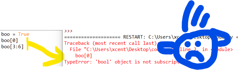
Consider the following minimal example where a TypeError: 'bool' object is not subscriptable occurs:
boo = True
boo[0]
# or:
boo[3:6]
This yields the following output:
Traceback (most recent call last): File "C:\Users\xcent\Desktop\code.py", line 2, in <module> boo[0]
TypeError: 'bool' object is not subscriptable
Solution Overview
Python raises the TypeError: 'bool' object is not subscriptable if you use indexing or slicing with the square bracket notation on a Boolean variable. However, the Boolean type is not indexable and you cannot slice it—it’s not iterable!
In other words, the Boolean class doesn’t define the __getitem__() method.
converting the Boolean to a string using the str() function because strings are subscriptable,
removing the indexing or slicing call,
defining a dummy __getitem__() method for a custom “Boolean wrapper class”.
Related Tutorials: Check out our tutorials on indexing and slicing on the Finxter blog to improve your skills!
Method 1: Convert Boolean to a String
If you want to access individual characters of the “Boolean” strings "True" and "False", consider converting the Boolean to a string using the str() built-in function. A string is subscriptable so the error will not occur when trying to index or slice the converted string.
A simple way to resolve this error is to put the Boolean into a list that is subscriptable—that is you can use indexing or slicing on lists that define the __getitem__() magic method.
You can also define your own wrapper type around the Boolean variable that defines a dunder method for __getitem__() so that every indexing or slicing operation returns a specified value as defined in the dunder method.
This hack is generally not recommended, I included it just for comprehensibility and to teach you something new.
Summary
The error message “TypeError: 'boolean' object is not subscriptable” happens if you access a boolean boo like a list such as boo[0] or boo[1:4]. To solve this error, avoid using slicing or indexing on a Boolean or use a subscriptable object such as lists or strings.
This is in continuation of our DeFi series. In this post, we look at yet another decentralized lending and borrowing platform Aave.
Full DeFi Course: Click the link to access our free full DeFi course that’ll show you the ins and outs of decentralized finance (DeFi).
Aave
Aave launched in 2017 is a DeFi protocol similar to Compound with a lot of upgrades.
Beyond what Compound provides, Aave gives several extra tokens for supply and borrowing. As of now, Compound offered nine different tokens (various ERC- 20 Ethereum- based assets).
Aave provides these nine besides an additional 13 that Compound does not.
Depositors give the market liquidity to generate a passive income, while borrowers can borrow if they have an over-collateralized token or can avail flash loans for under-collateralized (one-block liquidity).
Currently, we can see two major markets on Aave.
The first is for ERC-20 tokens that are more frequently used, like those of Compound, and their underlying assets, such as ETH, DAI and USDC.
The latter is only available with Uniswap LP tokens.
For instance, a user receives an LP token signifying market ownership when they deposit collateral into a liquidity pool on the Uniswap platform. To provide additional benefits, the LP tokens can be sold on the Uniswap market of Aave.
As per DeFi pulse, Aave has a TVL (Total Value Locked) of $4.09B as of today.
Fig: Defi Pulse for Aave
Aave Versions
Aave has released three versions (v1, v2 and v3) as of now and the Governance token of Aave is ‘AAVE’. Version 1 or v1 is the base version launched in 2017 and then there have been upgrades with multiple new features added. Below is a short comparison of when to use v2 or v3.
Fig: Aave borrow and lend (pic credit: https://docs.aave.com)
Borrow
You must deposit any asset to be used as collateral before borrowing.
The amount you can borrow up to depends on the value you have deposited and the readily available liquidity.
For instance, if there isn’t enough liquidity or if your health factor (minimum threshold of the collateral = 1, below this value, liquidation of your collateral is triggered) prevents it, you can’t borrow an asset.
The loan is repaid with the same asset that you borrowed.
For instance, if you borrow 1 ETH, you’ll need to pay back 1 ETH plus interest.
In the updated Version 2 of the Aave Protocol, you can also use your collateral to make payments. You can borrow any of the stable coins like USDC, DAI, USDT, etc. if you want to repay the loan based on the price of the USD.
Stable vs Variable Interest Rate
In the short-term, stable rates function as a fixed rate, but they can be rebalanced in the long run in reaction to alterations in the market environment. Depending on supply and demand in Aave, the variable rate can change.
The stable rate is the better choice for forecasting how much interest you will have to pay because, as its name suggests, it will remain fairly stable. The variable rate changes over time and, depending on market conditions, could be the optimal rate.
Through your dashboard, you can switch between the stable and variable rate at any time.
Deposit/Lending
Lenders share the interest payments made by borrowers based on the utilization rate multiplied by the average borrowing rate. The yield for depositors increases as reserve utilization increases.
Lenders are also entitled to a portion of the Flash Loan fees, equal to .09% of the Flash Loan volume.
There is no minimum or maximum deposit amount; you may deposit any amount you choose.
Flash Loans in Aave
Flash Loans are unique business agreements that let you borrow an asset as long as you repay the borrowed money (plus a fee) before the deal expires (also called One Block Borrows). Users are not required to provide collateral for these transactions in order to proceed.
Flash Loans have no counterpart in the real world, so understanding how state is controlled within blocks in blockchains is a prerequisite.
Flash-loan enables users to access pool liquidity for a single transaction as long as the amount borrowed plus fees are returned or (if permitted) a debt position is opened by the end of the transaction.
For flash loans, Aave V3 provides two choices:
(1) “flashLoan”: enables borrowers to access the liquidity of several reserves in a single flash loan transaction. In this situation, the borrower also has the choice to open a fixed or variable-rate loan position secured by provided collateral.
The fee for flashloan is waived for approved flash borrowers.
(2) “flashLoanSimple”: enables the borrower to access a single reserve’s liquidity for the transaction. For individuals looking to take advantage of a straightforward flash loan with a single reserve asset, this approach is gas-efficient.
The fee for flashloanSimple is not waived for the flash borrowers. The Flashloan fee on Aave V3 is 0.05%.
Let’s Code a Simple Flash Loan
Let’s code a simple flash loan in Aave, where we buy and repay the asset in the same transaction without having to provide any collateral. First, we set up the environment for writing the code.
Note: It is recommended to follow the video along for a better understanding.
$npm install -g truffle # in case truffle not installed
$mkdir aave_flashloan $cd aave_flashloan
$truffle init
$npm install @aave/core-v3
$npm install @openzeppelin/contracts
$npm install @openzeppelin/test-helpers
Note: Aave3 is currently available on Polygon, Arbitrum, Avalanche, and other L2 chains. As of now, it is not available on the Ethereum mainnet. Thus, we will fork the Polygon mainnet for our tests.
Set up a new app in Alchemy with the chain as Polygon mainnet and note down the API key.
This should run the flash loan test case, and it must pass.
Conclusion
This tutorial discussed Aave, a leading Dapp lending and borrowing provider.
It covered some basic functionalities supported in Aave, such as lending, borrowing, and flash loans.
There are many other features Aave supports and it is not possible to cover it in one post, such as governance, liquidation, and advanced features such as Siloed Borrowing, Credit Delegation, and many more.
The post also examined a simple flash loan contract using Aave API.
You can explore more about borrowing and lending with Aave in this link. It has a full stack Defi Aave dapp with frontend to perform borrowing and lending.
This article will show you how to retrieve a single generator element in Python. Before moving forward, let’s review what a generator does.
Quick Recap Generators
Definition Generator: A generator is commonly used when processing vast amounts of data. This function uses minimal memory and produces results in less time than a standard function.
Definition yield: The yield keyword returns a generator object instead of a value.
Definition next(): This function takes an iterator and an optional default value. Each time this function is called, it returns the next iterator item until all items are exhausted. Once exhausted, it returns the default value passed or a StopIteration Error.
Problem Formulation and Solution Overview
Question: How would we write code to retrieve and return a single element from a Generator?
We can accomplish this task by one of the following options:
Let’s say we want to start a weekly in-house lottery called LottoOne (yeah — the lottery naming doesn’t care about Python’s naming conventions ).
The code below will generate and return one (1) random element (an integer): the winning number for the week.
import random def LottoOne(): num = random.randint(1, 50) yield print(f'The Winning Number for the Week is: {num}!') gen = LottoOne()
next(gen)
The first line in the above code imports the random library. This library allows the generation of random numbers using the random.randint() function.
On the following line, an instance of LottoOne is instantiated and saved to the variable gen. If output to the terminal, an object similar to that shown below will display.
<generator object LottoOne at 0x00000236B9686880>
Since we only want the first randomly generated number, the code calls the next() function once and passes it one (1) argument, the object gen. The results are output to the terminal.
If you know what number you need to return from a generator, it can be referenced directly, as shown in the code below.
import itertools
from itertools import islice gen = (x for x in range(1, 50))
res = next(itertools.islice(gen, 2, None))
print(res)
The first two (2) lines in the above code import the itertools library and its associated function islice()needed to achieve the desired result.
The following line creates a generator comprehension using the range() function and passing it a start and stop position (1, 50-1). The results save to gen as an object.
If output to the terminal, an object similar to that shown below will display.
The default value. In this case, the keyword None. Passing a default value prevents a StopIteration error from occurring when the end of the iterator has been reached.
The results save to res and are output to the terminal.
3
The value of 3 can be found at index 2 in gen.
Method 3: Use a List, Generator Comprehension and slicing
gen = (i for i in range(1, 50))
res = list(gen)[3]
print(res)
The first line in the above code creates a Generator Comprehension using the range() function and passing it a start and stop position (1, 50-1). The results save to gen as an object.
If output to the terminal, an object similar to that shown below will display.
<generator object at 0x00000295D4DB78F0>
The following line converts the object to a list. Slicing is then applied to retrieve the list element at position three (3).
The results save to res and are output to the terminal.
4
The value of 4 can be found at index 3 in gen.
Method 4: Use a Generator and a For Loop
This example creates a Generator whose content is output to the terminal until a specific number is found.
def my_func(): yield 10 yield 20 yield 30 gen = my_func() for item in gen: if item == 20: print(item) break
This first line of the above code declares the function my_func(). This function will return, via a yield statement, a number (one/iteration).
Next, an object is declared and saved to gen.
If output to the terminal, an object similar to that shown below will display.
<generator object my_func at 0x0000022DE93D59A0>
The following line instantiates a for loop. This loop iterates through each yield statement in gen until the item contains a value of 20.
This value is output to the terminal, and the loop terminates via the break statement.
20
Summary
This article has provided four (4) ways to retrieve a single element from a Generator to select the best fit for your coding requirements.
Good Luck & Happy Coding!
Programming Humor – Python
“I wrote 20 short programs in Python yesterday. It was wonderful. Perl, I’m leaving you.” — xkcd
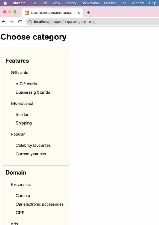
This PHP script will help if you want to display an Amazon-like product category tree. It will be useful for displaying the category menu in a hierarchical order, just like a tree.
The specialty of this PHP code is that it builds a multi-level category tree with infinite depth. It uses the recursion method to obtain this.
This is an initiator that calls the PHP recursive parsing to get the Category Tree HTML. In the PHP ZipArchive post, we used the same recursion concept to compress the contents of the enclosed directories.
Also, it has a UI holder to render the HTML hierarchical category menu.
A PHP class CategoryTree is created to read and parse the category array from the database.
This styles gives the category tree a pleasing look. Since it displays an infinite level of child categories, this CSS will help to rectify the default UI constraints.
Datatrans is one of the popular payment gateway systems in Europe for e-commerce websites. It provides frictionless payment solutions.
The Datatrans Payment gateway is widely popular in European countries. One of my clients from Germany required this payment gateway integrated into their online shop.
In this tutorial, I share the knowledge of integrating Datatrans in a PHP application. It will save the developers time to do research with the long-form documentation.
There are many integration options provided by this payment gateway.
Redirect and lightbox
Secure fields
Mobile SDK
API endpoints
In this tutorial, we will see the first integration option to set up the Datatrans payment gateway. We have seen many payment gateway integration examples in PHP in the earlier articles.
A working example follows helps to understand things easily. Before seeing the example, get the Datatrans merchant id and password. It will be useful for authentication purposes while accessing this payment API.
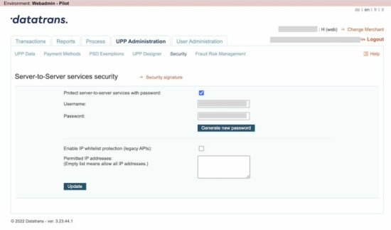
Get Datatrans merchant id and password
The following steps lead to getting the merchant id and password of your Datatrans account.
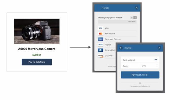
Get transaction id and proceed with payment via API
The initiate() function posts the amount to the PHP file to initiate Datatrans payment.
As the result, the PHP will return the transaction id to process the payment further.
The proceedPayment() function calls the Datatrans JavaScript API to start the payment. It will show a Datatrans overlay with card options to choose payment methods.
index.php (AJAX script to call Datatrans initiation)
Initiate payment transaction to get the Datatrans payment transaction id
This file is the PHP endpoint called via AJAX script to get the Datatrans transaction id.
It invokes the DatatransPaymentService to post the cURL request to the Datatrans API. It requested to initiate the payment and receives the transaction id from the Datatrans server.
This output will be read in the AJAX success callback to start the payment via the JavaScript library.
<HTML>
<HEAD>
<TITLE>Datatrans payment status notice</TITLE>
</HEAD>
<BODY> <div class="text-center">
<?php
if (! empty($_GET["status"])) { ?> <h1>Something wrong with the payment process!</h1> <p>Kindly contact admin with the reference of your transaction id <?php echo $_GET["datatransTrxId"]; ?></p>
<?php
} else { ?> <h1>Your order has been placed</h1> <p>We will contact you shortly.</p>
<?php
}
?>
</div>
</BODY>
</HTML>
The for loop ends naturally when all elements have been iterated over. After that, Python proceeds with the first statement after the loop construct.
The keyword break terminates a loop immediately. The program proceeds with the first statement after the loop construct.
The keyword continue terminates only the current loop iteration, but not the whole loop. The program proceeds with the first statement in the loop body.
You can see each of these three methods to terminate a for loop in the following graphic:
Let’s dive into each of those three approaches next!
Method 1: Visit All Elements in Iterator
The most natural way to end a Python for loop is to deplete the iterator defined in the loop expression for <var> in <iterator>. If the iterator’s next() method doesn’t return a value anymore, the program proceeds with the next statement after the loop construct. This immediately ends the loop.
Here’s an example that shows how the for loop ends as soon as all elements have been visited in the iterator returned by the range() function:
s = 'hello world' for c in range(5): print(c, end='') # hello
If the program executes a statement with the keyword break, the loop terminates immediately. No other statement in the loop body is executed and the program proceeds with the first statement after the loop construct. In most cases, you’d use the keyword break in an if construct to decide dynamically whether a loop should end, or not.
In the following example, we create a string with 11 characters and enter a for loop that ends prematurely after five iterations — using the keyword break in an if condition to accomplish that:
s = 'hello world' for i in range(10): print(s[i], end='') if i == 5: break # hello
As soon as the if condition evaluates to False, the break statement is executed—the loop ends.
The keyword continue terminates only the current loop iteration, but not the whole loop. The program proceeds with the first statement in the loop body. The most common use of continue is to avoid the execution of certain parts of the loop body, constrained by a condition checked in an if construct.
Here’s an example:
for i in range(10): if i == 5: break else: continue print('NEVER EXECUTED')
Python iterates over an iterator with 10 elements. However, in each iteration, it either ends the loop using break or continues with the next iteration using continue.
However, the remaining loop body that actually does something such as printing'NEVER EXECUTED' is, well, never executed.
Python Keywords Cheat Sheet
You can learn about the most important Python keywords in this concise cheat sheet—if you’re like me, you love cheat sheets as well!
You can download it here:
Summary
You’ve learned three ways to terminate a while loop.
Method 1: The for loop terminates automatically after all elements have been visited. You can modify the iterator using the __next__() dunder method.
Method 2: The keyword break terminates a loop immediately. The program proceeds with the first statement after the loop construct.
Method 3: The keyword continue terminates only the current loop iteration, but not the whole loop. The program proceeds with the first statement in the loop body.
Thanks for reading this tutorial—if you want to boost your Python skills further, I’d recommend you check out my free email academy and download the free Python lessons and cheat sheets here:
Join us, it’s fun!
Programmer Humor
Question: How did the programmer die in the shower? ☠
❗ Answer: They read the shampoo bottle instructions: Lather. Rinse. Repeat.
Some time ago, we discovered how to send an email with Python using smtplib, a built-in email module. Back then, the focus was made on the delivery of different types of messages via SMTP server. Today, we prepared a similar tutorial but for Django.
This popular Python web framework allows you to accelerate email delivery and make it much easier. And these code samples of sending emails with Django are going to prove that.
A simple code example of how to send an email
Let’s start our tutorial with a few lines of code that show you how simple it is to send an email in Django. Import send_mail in the beginning of the file:
from django.core.mail import send_mail
And call the code below in the necessary place.
send_mail( 'That’s your subject', 'That’s your message body', 'from@yourdjangoapp.com', ['to@yourbestuser.com'], fail_silently=False,
)
These lines are enclosed in the django.core.mail module that is based on smtplib. The message delivery is carried out via SMTP host, and all the settings are set by default:
EMAIL_HOST is different for each email provider you use. For example, if you have a Gmail account and use their SMTP server, you’ll have EMAIL_HOST = ‘smtp.gmail.com’.
Also, validate other values that are relevant to your email server. Eventually, you need to choose the way to encrypt the mail and protect your user account by setting the variable EMAIL_USE_TLS or EMAIL_USE_SSL.
If you have an email provider that explicitly tells you which option to use, then it’s clear. Otherwise, you may try different combinations using True and False operators. Note that only one of these options can be set to True.
EMAIL_BACKEND tells Django which custom or predefined email backend will work with.
EMAIL_HOST. You can set up this parameter as well.
SMTP email backend
In the example above, EMAIL_BACKEND is specified as django.core.mail.backends.smtp.EmailBackend. It is the default configuration that uses SMTP server for email delivery. Defined email settings will be passed as matching arguments to EmailBackend.
django.core.mail.backends.console.EmailBackend– the console backend that composes the emails that will be sent to the standard output. Not intended for production use.
django.core.mail.backends.filebased.EmailBackend – the file backend that creates emails in the form of a new file per each new session opened on the backend. Not intended for production use.
django.core.mail.backends.locmem.EmailBackend– the in-memory backend that stores messages in the local memory cache of django.core.mail.outbox. Not intended for production use.
django.core.mail.backends.dummy.EmailBackend – the dummy cache backend that implements the cache interface and does nothing with your emails. Not intended for production use.
Any out-of-the-box backend for Amazon SES, Mailgun, SendGrid, and other services.
How to send emails via SMTP
Once you have that configured, all you need to do to send an email is to import the send_mail or send_mass_mailfunction from django.core.mail. These functions differ in the connection they use for messages. send_mailuses a separate connection for each message. send_mass_mailopens a single connection to the mail server and is mostly intended to handle mass emailing.
Sending email with send_mail
This is the most basic function for email delivery in Django. It comprises four obligatory parameters to be specified: subject, message, from_email, and recipient_list.
In addition to them, you can adjust the following:
auth_user: If EMAIL_HOST_USER has not been specified, or you want to override it, this username will be used to authenticate to the SMTP server.
auth_password: If EMAIL_HOST_PASSWORD has not been specified, this password will be used to authenticate to the SMTP server.
connection: The optional email backend you can use without tweaking EMAIL_BACKEND.
html_message: Lets you send multipart emails.
fail_silently: A boolean that controls how the backend should handle errors. If True – exceptions will be silently ignored. If False – smtplib.SMTPException will be raised.
Other functions for email delivery include mail_admins and mail_managers. Both are shortcuts to send emails to the recipients predefined in ADMINS and MANAGERS settings respectively.
For them, you can specify such arguments as subject, message, fail_silently, connection, and html_message.
The from_email argument is defined by the SERVER_EMAIL setting.
What is EmailMessage for?
If the email backend handles the email sending, the EmailMessage class answers for the message creation. You’ll need it when some advanced features like BCC or an attachment are desirable. That’s how an initialized EmailMessage may look:
from django.core.mail import EmailMessage
email = EmailMessage( subject = 'That’s your subject', body = 'That’s your message body', from_email = 'from@yourdjangoapp.com', to = ['to@yourbestuser.com'], bcc = ['bcc@anotherbestuser.com'], reply_to = ['whoever@itmaybe.com'],
)
In addition to the EmailMessage objects you can see in the example, there are also other optional parameters:
connection: defines an email backend instance for multiple messages.
attachments: specifies the attachment for the message.
headers: specifies extra headers like Message-ID or CC for the message.
cc: specifies email addresses used in the “CC” header.
The methods you can use with the EmailMessage class are the following:
send: get the message sent.
message: composes a MIME object (django.core.mail.SafeMIMEText or django.core.mail.SafeMIMEMultipart).
recipients: returns a list of the recipients specified in all the attributes including to, cc, and bcc.
attach: creates and adds a file attachment. It can be called with a MIMEBase instance or a triple of arguments consisting of filename, content, and mime type.
attach_file: creates an attachment using a file from a filesystem. We’ll talk about adding attachments a bit later.
How to send multiple emails
To deliver a message via SMTP, you need to open a connection and close it afterwards. This approach is quite awkward when you need to send multiple transactional emails. Instead, it is better to create one connection and reuse it for all messages.
This can be done with the send_messages method that the email backend API has. Check out the following example:
from django.core import mail
connection = mail.get_connection()
connection.open()
email1 = mail.EmailMessage( 'That’s your subject', 'That’s your message body', 'from@yourdjangoapp.com', ['to@yourbestuser1.com'], connection=connection,
)
email1.send()
email2 = mail.EmailMessage( 'That’s your subject #2', 'That’s your message body #2', 'from@yourdjangoapp.com', ['to@yourbestuser2.com'],
)
email3 = mail.EmailMessage( 'That’s your subject #3', 'That’s your message body #3', 'from@yourdjangoapp.com', ['to@yourbestuser3.com'],
)
connection.send_messages([email2, email3])
connection.close()
What you can see here is that the connection was opened for email1, and send_messages uses it to send emails #2 and #3. After that, you close the connection manually.
How to send multiple emails with send_mass_mail
send_mass_mail is another option to use only one connection for sending different messages.
message1 = ('That’s your subject #1', 'That’s your message body #1', 'from@yourdjangoapp.com', ['to@yourbestuser1.com', 'to@yourbestuser2.com'])
message2 = ('That’s your subject #2', 'That’s your message body #2', 'from@yourdjangoapp.com', ['to@yourbestuser2.com'])
message3 = ('That’s your subject #3', 'That’s your message body #3', 'from@yourdjangoapp.com', ['to@yourbestuser3.com'])
send_mass_mail((message1, message2, message3), fail_silently=False)
Each email message contains a datatuple made of subject, message, from_email, and recipient_list. Optionally, you can add other arguments that are the same as for send_mail.
How to send an HTML email
All versions starting from 1.7 let you send an email with HTML content using send_mail like this:
from django.core.mail import send_mail
subject = 'That’s your subject'
html_message = render_to_string('mail_template.html', {'context': 'values'})
plain_message = strip_tags(html_message)
from_email = 'from@yourdjangoapp.com>'
to = 'to@yourbestuser.com'
mail.send_mail(subject, plain_message, from_email, [to], html_message=html_message)
Older versions users will have to mess about with EmailMessage and its subclass EmailMultiAlternatives. It lets you include different versions of the message body using the attach_alternative method. For example:
from django.core.mail import EmailMultiAlternatives
subject = 'That’s your subject'
from_email = 'from@yourdjangoapp.com>'
to = 'to@yourbestuser.com'
text_content = 'That’s your plain text.'
html_content = '<p>That’s <strong>the HTML part</strong></p>'
message = EmailMultiAlternatives(subject, text_content, from_email, [to])
message.attach_alternative(html_content, "text/html")
message.send()
How to send an email with attachments
In the EmailMessage section, we’ve already mentioned sending emails with attachments. This can be implemented using attach or attach_file methods.
The first one creates and adds a file attachment through three arguments – filename, content, and mime type.
The second method uses a file from a filesystem as an attachment. That’s how each method would look like in practice:
You’re not limited to the abovementioned email backend options and can tailor your own. For this, you can use standard backends as a reference. Let’s say, you need to create a custom email backend with the SMTP_SSL connection support required to interact with Amazon SES.
The default SMTP backend will be the reference. First, add a new email option to settings.py.
Make sure that you are allowed to send emails with Amazon SES using these AWS_ACCESS_KEY_ID and AWS_SECRET_ACCESS_KEY (or error message will tell you about it :D)
Then create a file your_project_name/email_backend.py with the following content:
import boto3
from django.core.mail.backends.smtp import EmailBackend
from django.conf import settings
class SesEmailBackend(EmailBackend): def __init__( self, fail_silently=False, **kwargs ): super().__init__(fail_silently=fail_silently) self.connection = boto3.client( 'ses', aws_access_key_id=settings.AWS_ACCESS_KEY_ID, aws_secret_access_key=settings.AWS_SECRET_ACCESS_KEY, region_name=settings.AWS_REGION, ) def send_messages(self, email_messages): for email_message in email_messages: self.connection.send_raw_email( Source=email_message.from_email, Destinations=email_message.recipients(), RawMessage={"Data": email_message.message().as_bytes(linesep="\r\n")} )
This is the minimum needed to send an email using SES. Surely you will need to add some error handling, input sanitization, retries etc. but this is out of our topic.
You might see that we have imported boto3 in the beginning of the file. Don’t forget to install it using a command
pip install boto3
It’s not necessary to reinvent the wheel every time you need a custom email backend. You can find already existing libraries, or just receive SMTP credentials in your Amazon console and use the default email backend. It’s just about figuring out the best option for you and your project.
Sending emails using SES from Amazon
So far, you can benefit from several services that allow you to send transactional emails at ease. If you can’t choose one, check out our blog post about Sendgrid vs. Mandrill vs. Mailgun. It will help a lot. At this point, Mailtrap has launched its own sending solution.
So, you could easily start sending transactional emails in Django using our guide. But today, we’ll discover how to make your Django app send emails via Amazon SES. It is one of the most popular services so far. Besides, you can take advantage of a ready-to-use Django email backend for this service – django-ses.
Set up the library
You need to execute pip install django-ses to install django-ses. Once it’s done, tweak your settings.py with the following line:
EMAIL_BACKEND = 'django_ses.SESBackend'
AWS credentials
Don’t forget to set up your AWS account to get the required credentials – AWS access keys that consist of access key ID and secret access key.
For this, add a user in Identity and Access Management (IAM) service.
Then, choose a user name and Programmatic access type. Attach AmazonSESFullAccess permission and create a user. Once you’ve done this, you should see AWS access keys. Update your settings.py:
Now, you can send your emails using django.core.mail.send_mail:
from django.core.mail import send_mail
send_mail( 'That’s your subject', 'That’s your message body', 'from@yourdjangoapp.com', ['to@yourbestuser.com']
)
django-ses is not the only preset email backend you can leverage. At the end of this article, you’ll find more useful libraries to optimize email delivery of your Django app. But first, a step you should never send emails without.
Testing email sending in Django
Once you’ve got everything prepared for sending email messages, it is necessary to do some initial testing of your mail server. In Python, this can be done with one command:
This allows you to send emails to your local SMTP server. The DebuggingServer feature won’t actually send the email but will let you see the content of your message in the shell window. That’s an option you can use off-hand.
Django’s TestCase
TestCase is a solution to test a few aspects of your email delivery. It uses locmem.EmailBackend, which, as you remember, stores messages in the local memory cache – django.core.mail.outbox. So, this test runner does not actually send emails. Once you’ve selected this email backend
you can use the following unit test sample to test your email sending capability.
from django.core import mail
from django.test import TestCase
class EmailTest(TestCase): def test_send_email(self): mail.send_mail( 'That’s your subject', 'That’s your message body', 'from@yourdjangoapp.com', ['to@yourbestuser.com'], fail_silently=False, ) self.assertEqual(len(mail.outbox), 1) self.assertEqual(mail.outbox[0].subject, 'That’s your subject') self.assertEqual(mail.outbox[0].body, 'That’s your message body')
This code will test not only your email sending but also the correctness of the email subject and message body.
Testing with Mailtrap
Mailtrap can be a rich solution for testing. First, it lets you test not only the SMTP server but also the email content and do other essential checks from the email testing checklist. Second, it is a rather easy-to-use tool.
All you need to do is to copy the SMTP credentials from your demo inbox and tweak your settings.py. Or you can just copy/paste these four lines from the Integrations section by choosing Django in the pop-up menu.
If there is no message in the Mailtrap Demo inbox or there are some issues with HTML content, you need to polish your code.
Django email libraries to simplify your life
As a conclusion to this blog post about sending emails with Django, we’ve included a brief introduction of a few libraries that will facilitate your email workflow.
django-anymail
This is a collection of email backends and webhooks for numerous famous email services including SendGrid, Mailgun, and others. django-anymail works with the django.core.mail module and normalizes the functionality of transactional email service providers.
django-mailer
django-mailer is a Django app you can use to queue email sending. With it, scheduling your emails is much easier.
django-post_office
With this app, you can send and manage your emails. django-post_office offers many cool features like asynchronous email sending, built-in scheduling, multiprocessing, etc.
django-templated-email
This app is about sending templated emails. In addition to its own functionalities, django-templated-email can be used in tow with django-anymail to integrate transactional email service providers.
How to receive emails in Django
To receive emails in Django, it is better to use the django-mailbox development library if you need to import messages from local mailboxes, POP3, IMAP, or directly receive messages from Postfix or Exim4.
While using Django-mailbox, mailbox functions as a message queue that is being gradually processed. The library helps retrieve email messages and then erases them so they are not downloaded again the next time.
Mailbox types supported by django-mailbox: POP3, IMAP, Gmail IMAP with Oauth2 authentication, local file-based mailboxes like Maildir, Mbox, Babyl, MH, or MMDF.
Here’s a step-by-step guide on how to quickly set up your Django-mailbox and start receiving emails.
git clone https://github.com/coddingtonbear/django-mailbox.git
cd django-mailbox
python setup.py install
After installing the package, go to settings.py file of the django project and add django_mailboxto INSTALLED_APPS.
Then, run python manage.py migrate django_mailbox from your project file to create the necessary database tables.
Finally, go to your project’s Django Admin and create a mailbox to consume.
Don’t forget to verify if your mailbox was set up right. You can do that from a shell opened to your project’s directory, using the getmail command running python manage.py getmail
When you are done with the installation and checking the configurations, it’s time to receive incoming emails. There are five different ways to do that.
In your code
Use the get_new_mail method to collect new messages from the server.
With Django Admin
Go to Django Admin, then to ‘Mailboxes’ page, check all the mailboxes you need to receive emails from. At the top of the list with mailboxes, choose the action selector ‘Get new mail’ and click ‘Go’.
With cron job
Run the management command getmail in python manage.py getmail
Directly from Exim4
To configure Exim4 to receive incoming mail begin with adding a new router:
In case the email addresses you are trying to add are handled by other routers, disable them. For this change, the contents of local_parts must match a colon-delimited list of usernames for which you would like to receive mail.
5. Directly from Postfix
With Postfix get new mail to a script using pipe. The steps to set up receiving incoming mail directly from Postfix are pretty much the same as with Exim4. However, you might need to check out the Postfix pipe documentation.
There’s also an option to subscribe to the incoming django-mailbox signal if you need to process your incoming mail at the time that suits you best.
Use this piece of code to do that:
from django_mailbox.signals import message_received
from django.dispatch import receiver @receiver(message_received)
def dance_jig(sender, message, **args): print "I just received a message titled %s from a mailbox named %s" % (message.subject, message.mailbox.name, )
Keep in mind that this should be loaded to models.py or elsewhere early enough for the signal not to be fired before your signal handler’s registration is processed.
We hope that you find our guide helpful and the list of packages covered help facilitate your email workflow. You can always find more apps at Django Packages.
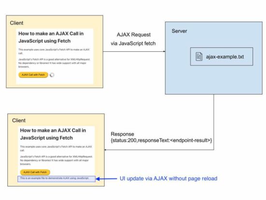
This is a pure JavaScript solution to use AJAX without jQuery or any other third-party plugins.
The AJAX is a way of sending requests to the server asynchronously from a client-side script. In general, update the UI with server response without reloading the page.
I present two different methods of calling backend (PHP) with JavaScript AJAX.
via XMLHTTPRequest.
using JavaScript fetch prototype.
This tutorial creates simple examples of both methods. It will be an easy start for beginners of AJAX programming. It simply reads the content of a .txt file that is in the server via JavaScript AJAX.
The below script has the following AJAX lifecycle to get the response from the server.
It instantiates XMLHttpRequest class.
It defines a callback function to handle the onreadystatechange event.
It prepares the AJAX request by setting the request method, server endpoint and more.
Calls send() with the reference of the XMLHttpRequest instance.
In the onreadystatechange event, it can read the response from the server. This checks the HTTP response code from the server and updates the UI without page refresh.
During the AJAX request processing, it shows a loader icon till the UI gets updated with the AJAX response data.
ajax-xhr.php
<!DOCTYPE html>
<html>
<head>
<title>How to make an AJAX Call in JavaScript with Example</title>
<link rel='stylesheet' href='style.css' type='text/css' />
<link rel='stylesheet' href='form.css' type='text/css' />
<style>
#loader-icon { display: none;
}
</style>
</head>
<body> <div class="phppot-container"> <h1>How to make an AJAX Call in JavaScript</h1> <p>This example uses plain JavaScript to make an AJAX call.</p> <p>It uses good old JavaScript's XMLHttpRequest. No dependency or libraries!</p> <div class="row"> <button onclick="loadDocument()">AJAX Call</button> <div id="loader-icon"> <img src="loader.gif" /> </div> </div> <div id='ajax-example'></div> <script> function loadDocument() { document.getElementById("loader-icon").style.display = 'inline-block'; var xmlHttpRequest = new XMLHttpRequest(); xmlHttpRequest.onreadystatechange = function() { if (xmlHttpRequest.readyState == XMLHttpRequest.DONE) { document.getElementById("loader-icon").style.display = 'none'; if (xmlHttpRequest.status == 200) { // on success get the response text and // insert it into the ajax-example DIV id. document.getElementById("ajax-example").innerHTML = xmlHttpRequest.responseText; } else if (xmlHttpRequest.status == 400) { // unable to load the document alert('Status 400 error - unable to load the document.'); } else { alert('Unexpected error!'); } } }; xmlHttpRequest.open("GET", "ajax-example.txt", true); xmlHttpRequest.send(); }
</script> </body>
</html>
Using JavaScript fetch prototype
This example calls JavaScript fetch() method by sending the server endpoint URL as its argument.
This method returns the server response as an object. This response object will contain the status and the response data returned by the server.
As like in the first method, it checks the status code if the “response.status” is 200. If so, it updates UI with the server response without reloading the page.
ajax-fetch.php
<!DOCTYPE html>
<html>
<head>
<title>How to make an AJAX Call in JavaScript using Fetch API with Example</title>
<link rel='stylesheet' href='style.css' type='text/css' />
<link rel='stylesheet' href='form.css' type='text/css' />
<style>
#loader-icon { display: none;
}
</style>
</head>
<body> <div class="phppot-container"> <h1>How to make an AJAX Call in JavaScript using Fetch</h1> <p>This example uses core JavaScript's Fetch API to make an AJAX call.</p> <p>JavaScript's Fetch API is a good alternative for XMLHttpRequest. No dependency or libraries! It has wide support with all major browsers.</p> <div class="row"> <button onclick="fetchDocument()">AJAX Call with Fetch</button> <div id="loader-icon"> <img src="loader.gif" /> </div> </div> <div id='ajax-example'></div> <script> async function fetchDocument() { let response = await fetch('ajax-example.txt'); document.getElementById("loader-icon").style.display = 'inline-block'; console.log(response.status); console.log(response.statusText); if (response.status === 200) { document.getElementById("loader-icon").style.display = 'none'; let data = await response.text(); document.getElementById("ajax-example").innerHTML = data; } }
</script> </body>
</html>
An example use case scenarios of using AJAX in an application
AJAX is a powerful tool. It has to be used in an effective way wherever needed.
The following are the perfect example scenarios of using AJAX in an application.
To update the chat window with recent messages.
To have the recent notification on a social media networking website.
To update the scoreboard.
To load recent events on scroll without page reload.

 Question: Given a Boolean value
  Recommended Tutorial: String to Boolean Conversion
 This is because all Python objects are “truthy”, i.e., they have an associated Boolean value. As a rule of thumb: empty values return Boolean


 As a rule of thumb, the order should be one plus the total number of (trending) hills + peaks in the graph, but not much more than that.


 Related Tutorials: Check out our tutorials on


 Note: It is recommended to follow the video along for a better understanding.
 ).
).