Wait is there every aspect of human life. Let’s get philosophical for a moment! For every good thing in life, you need to wait.
“There’s no such thing as failure – just waiting for success.” – John Osborne
Like in life, wait in programming is also unavoidable. It is a tool, that you will need some day on desperate situations. For example, a slider, a fading animation, a bouncing ball, you never know.
In this tutorial, we will learn about how to wait one second in JavaScript? One second is an example. It could be a “5 seconds” or any duration your code needs to sleep before continuing with operation.
Refer this linked article to learn about PHP sleep.
JavaScript wait 1 second
I have used the good old setTimeout JavaScript function to wait. It sleeps the processing for the milliseconds duration set. Then calls the callback function passed.
You should put the code to execute after wait inside this callback function. As for the wait duration 1000 millisecond is one second. If you want to wait 5 seconds, then pass 5000.
This code will be handy if you are creating a news ticker like scroll animation.
If you are using a modern browser, then you can use the below code. Modern means, your browser should support ES6 JavaScript standard.
In summary, you need support for JavaScript Promise. Here we use the setTimeout function. It resolves the promise after the defined milliseconds wait.
// Promise is available with JavaScript ES6 standard
// Need latest browsers to run it
const wait = async (milliseconds) => { await new Promise(resolve => { return setTimeout(resolve, milliseconds) });
}; const testWait = async () => { console.log('Before wait.'); await wait(1000); console.log('After wait.');
} testWait();
JavaScript wait 1 second in loop
If you want to wait the processing inside a loop in JavaScript, then use the below code. It uses the above Promise function and setTimeout to achieve the wait.
If yours is an old browser then use the first code given above for the wait part. If you need to use this, then remember to read the last section of this tutorial. In particular, if you want to “wait” in a mission critical JavaScript application.
const wait = async (milliseconds) => { await new Promise(resolve => { return setTimeout(resolve, milliseconds) });
}; const waitInLoop = async () => { for (let i = 0; i < 10; i++) { console.log('Waiting ...'); await wait(1000); console.log(i); } console.log("The wait is over.");
} waitInLoop();
JavaScript wait 1 second in jQuery
This is for people out there who wishes to write everything in jQuery. It was one of the greatest frontend JavaScript libraries but nowadays losing popularity. React is the new kid in the block. Here in this wait scenario, there is no need to look for jQuery specific code even if you are in jQuery environment.
Because you will have support for JavaScript. You can use setTimeout without any jQuery specific constructs. I have wrapped setTimeout in a jQuery style code. Its old wine in a new bottle.
// if for some strange reason you want to write // it in jQuery style // just wrapping the setTimout function in jQuery style $.wait = function(callback, milliseconds) { return window.setTimeout(callback, milliseconds); } $.wait(function() { $("#onDiv").slideUp() }, 1000);
Cancel before wait for function to finish
You may have to cancel the wait and re-initiate the setTimeout in special scenarios. In such a situation use the clearTimeout() function as below. Go through the next section to know about such a special wait scenario.
let timeoutId = setTimeout(() => { // do process }) // store the timeout id and call clearTimeout() function // to clear the already set timeout clearTimeout(timeoutId);
Is the wait real?
You need to understand what the JavaScript wait means. When the JavaScript engine calls setTimeout, it processes a function. When the function exits, then a timeout with defined milliseconds is set. After that wait, then JavaScript engine makes the callback.
When you want to know the total wait period for next consecutive call. You need to add the time taken by your function to process to the wait duration.
So that is a variable unit. Assume that the function runs for five seconds. And the setTimeout wait duration is one second. Then the actual wait will become six seconds for the next call.
If you want to precise call every five seconds, then you need to define a self adjusting setTimeout timer.
You should account the time taken to process, then reduce the time from the wait milliseconds. Then cancel the current setTimeout. And start new setTimeout with the new calculated time.
That’s going to be tricky. If you are running a mission critical wait call, then that is the way to go.
For example, general UI animations, the above basic implementations will hold good. But you need the self adjusting setTimeout timer for critical time based events.
setInterval will come closer for the above scenario. Any other UI process running in main thread will affect setInterval’s wait period. Then your one second wait may get converted to 5 seconds wait. So, you should define a self adjusting setTimeout wait for mission critical events.
Here you will find additional examples of Plotly Dash components, layouts and style. To learn more about making dashboards with Plotly Dash, and how to buy your copy of “The Book of Dash”, please see the reference section at the bottom of this article.
As you read the article, feel free to run the explainer video on the Card components from one of our coauthors’ “Charming Data” YT channel:
This article will focus on the Card components from the Dash Boostrap Component library. Using cards is a great way to create eye-catching content. We’ll show you how to make the card content interactive with callbacks, but first we’ll focus on the style and layout.
Plotly Dash App with a Bootstrap Card
We’ll start with the basics – a minimal Dash app to display a single card without any additional styling. Be sure to check out the complete reference for using Dash Bootstrap cards.
Next, we’ll show how to jazz it up to make it look better — and more importantly — so it conveys key information at a glance.
from dash import Dash, html
import dash_bootstrap_components as dbc app = Dash(__name__, external_stylesheets=[dbc.themes.SPACELAB, dbc.icons.BOOTSTRAP]) card = dbc.Card( dbc.CardBody( [ html.H1("Sales"), html.H3("$104.2M") ], ),
) app.layout=dbc.Container(card) if __name__ == "__main__": app.run_server(debug=True)
Styling a Dash Bootstrap Card
An easy way to style content is by using Boostrap utility classes. See all the utility classes at the Dash Bootstrap Cheatsheet app. This handy cheatsheet is made by a co-author of “The Book of Dash”.
In this card, we center the text and change the color with “text-center” and “text-success“. The Bootstrap themes have named colors and “success” is a shade of green.
Recommended Resource: For more information about styling your app with a Boostrap theme, see Dash Bootstrap Theme Explorer
Feel free to watch Adam’s explainer video on Bootstrap and styling your app if you need to get up to speed!
Dash Bootstrap Card with Icons
You can add Bootstrap and/or Font Awesome icons to your Dash Bootstrap components. In this example, we will add the bank icon as well as change the background color using the Bootstrap utility class bg-primary.
To learn more, see the Icons section of the dash-bootstrap-components documentation. You can also find more information about adding icons to dash components in the buttons article.
In business intelligence dashboards, it’s common to highlight KPIs or Key Performance Indicators in a group of cards. You can find many examples in the Plotly App Gallery:
This app places three KPI cards side-by-side. We use the dbc.Row and dbc.Col components to create this responsive card layout. When you run this app, try changing the width of the browser window to see how the cards expand to fill the row based on the screen size.
This app also demonstrates the usage of Bootstrap border utility classes to add and style a border. Here we add a border on the left and change the color to highlight the results. Another trick is to use the “text-nowrap” class to keep the icon and the text together on the same line when the cards shrink to accommodate small screen sizes.
In the previous example, notice that a lot of the code for creating the card is the same. To reduce the amount of repetitive code, let’s create cards in a function.
In this app, we introduce the dbc.CardHeader component and the "shadow" class to style the card. We’ll show you how to add more style later in the app that displays crypto prices.
from dash import Dash, html
import dash_bootstrap_components as dbc app = Dash(__name__, external_stylesheets=[dbc.themes.SPACELAB]) summary = {"Sales": "$100K", "Profit": "$5K", "Orders": "6K", "Customers": "300"} def make_card(title, amount): return dbc.Card( [ dbc.CardHeader(html.H2(title)), dbc.CardBody(html.H3(amount, id=title)), ], className="text-center shadow", ) app.layout = dbc.Container( dbc.Row([dbc.Col(make_card(k, v)) for k, v in summary.items()], className="my-4"), fluid=True,
) if __name__ == "__main__": app.run_server(debug=True)
Dash Bootstrap Card with an Image
This card uses the dbc.CardImage component. This is a great format for the “who’s who” section of your app. It works well for displaying information about products too.
from dash import Dash, html
import dash_bootstrap_components as dbc app = Dash(__name__, external_stylesheets=[dbc.themes.SPACELAB]) count = "https://user-images.githubusercontent.com/72614349/194616425-107a62f9-06b3-4b84-ac89-2c42e04c00ac.png" card = dbc.Card([ dbc.CardImg(src=count, top=True), dbc.CardBody( [ html.H3("Count von Count", className="text-primary"), html.Div("Chief Financial Officer"), html.Div("Sesame Street, Inc.", className="small"), ] )], className="shadow my-2", style={"maxWidth": 350},
) app.layout=dbc.Container(card) if __name__ == "__main__": app.run_server(debug=True)
Dash Bootstrap Card with an Image and a Link
This app has a card with the dbc.CardLink component.
When you run this app, try clicking on either the logo or the title. You will see that both are links to the Plotly site displaying the current job openings.
We do this by including both the html.Img component with the Plotly logo and the html.Span with the title in the dbc.CardLink component.
This app puts the image in the background and uses the dbc.CardImgOverlay component to place content on top of the image.
We also use dbc.Buttons to link to other sites for more information. See the buttons article for more information. Be sure to run the app and check out the links. The Webb Telescope app is pretty cool!
from dash import Dash, html
import dash_bootstrap_components as dbc app = Dash(__name__, external_stylesheets=[dbc.themes.SPACELAB, dbc.icons.BOOTSTRAP]) webb_deep_field = "https://user-images.githubusercontent.com/72614349/192781103-2ca62422-2204-41ab-9480-a730fc4e28d7.png"
card = dbc.Card( [ dbc.CardImg(src=webb_deep_field), dbc.CardImgOverlay([ html.H2("James Webb Space Telescope"), html.H3("First Images"), html.P( "Learn how to make an app to compare before and after images of Hubble vs Webb with ~40 lines of Python", style={"marginTop":175}, className="small", ), dbc.Button("See the App", href="https://jwt.pythonanywhere.com/"), dbc.Button( [html.I(className="bi bi-github me-2"), "source code"], className="ms-2 text-white", href="https://github.com/AnnMarieW/webb-compare", ) ]) ], style={"maxWidth": 500}, className="my-4 text-center text-white"
) app.layout=dbc.Container(card) if __name__ == "__main__": app.run_server(debug=True)
This app shows live updates of crypto prices. We use a dcc.Interval component to fetch the data from CoinGecko every 6 seconds.
The CoinGecko API is easy to use because you don’t need an API key, and it’s free if you keep the number of updates within the free tier limits. We pull the current price, 24 hour price change, and the coin logo from the data feed and display the data in a nicely styled card.
In this app we introduce callbacks to update the data, and show how to get the data from CoinGecko. All the other styling has been covered in previous examples.
Note that in this app, the color of the text and the up and down arrows are updated dynamically based on the data in the make_card function.
import dash
from dash import Dash, dcc, html, Input, Output
import dash_bootstrap_components as dbc
import requests app = Dash(__name__, external_stylesheets=[dbc.themes.SUPERHERO, dbc.icons.BOOTSTRAP]) coins = ["bitcoin", "ethereum", "binancecoin", "ripple"]
interval = 6000 # update frequency - adjust to keep within free tier
api_url = "https://api.coingecko.com/api/v3/coins/markets?vs_currency=usd" def get_data(): try: response = requests.get(api_url, timeout=1) return response.json() except requests.exceptions.RequestException as e: print(e) def make_card(coin): change = coin["price_change_percentage_24h"] price = coin["current_price"] color = "danger" if change < 0 else "success" icon = "bi bi-arrow-down" if change < 0 else "bi bi-arrow-up" return dbc.Card( html.Div( [ html.H4( [ html.Img(src=coin["image"], height=35, className="me-1"), coin["name"], ] ), html.H4(f"${price:,}"), html.H5( [f"{round(change, 2)}%", html.I(className=icon), " 24hr"], className=f"text-{color}", ), ], className=f"border-{color} border-start border-5", ), className="text-center text-nowrap my-2 p-2", ) mention = html.A( "Data from CoinGecko", href="https://www.coingecko.com/en/api", className="small"
)
interval = dcc.Interval(interval=interval)
cards = html.Div()
app.layout = dbc.Container([interval, cards, mention], className="my-5") @app.callback(Output(cards, "children"), Input(interval, "n_intervals"))
def update_cards(_): coin_data = get_data() if coin_data is None or type(coin_data) is dict: return dash.no_update # make a list of cards with updated prices coin_cards = [] updated = None for coin in coin_data: if coin["id"] in coins: updated = coin.get("last_updated") coin_cards.append(make_card(coin)) # make the card layout card_layout = [ dbc.Row([dbc.Col(card, md=3) for card in coin_cards]), dbc.Row(dbc.Col(f"Last Updated {updated}")), ] return card_layout if __name__ == "__main__": app.run_server(debug=True)
Plotly Dash App with a Sidebar
A common layout for Dash apps is to put inputs in a sidebar, and the output in the main section of the page. We can place both the sidebar and the output in Dash Boostrap Card components.
TypeError: 'dict_keys' object is not subscriptable
You’re not alone! This short tutorial will show you why this error occurs, how to fix it, and how to never make the same mistake again.
So, let’s get started!
Solution
Python raises the “TypeError: 'dict_keys' object is not subscriptable” if you use indexing or slicing on the dict_keys object obtained with dict.keys(). To solve the error, convert the dict_keys object to a list such as in list(my_dict.keys())[0].
print(list(my_dict.keys())[0])
Example
The following minimal example that leads to the error:
d = {1:'a', 2:'b', 3:'c'}
print(d.keys()[0])
Output:
Traceback (most recent call last): File "C:\Users\...\code.py", line 2, in <module> print(d.keys()[0])
TypeError: 'dict_keys' object is not subscriptable
Note that the same error message occurs if you use slicing instead of indexing:
d = {1:'a', 2:'b', 3:'c'}
print(d.keys()[:-1]) # <== same error
Fixes
The reason this error occurs is that the dictionary.keys() method returns a dict_keys object that is not subscriptable.
You can use the type() function to check it for yourself:
print(type(d.keys()))
# <class 'dict_keys'>
Note: You cannot expect dictionary keys to be ordered, so using indexing on a non-ordered type wouldn’t make too much sense, would it?
You can fix the non-subscriptable TypeError by converting the non-indexable dict_keys object to an indexable container type such as a list in Python using the list() or tuple() function.
Here’s an example fix:
d = {1:'a', 2:'b', 3:'c'}
print(list(d.keys())[0])
# 1
Here’s an other example fix:
d = {1:'a', 2:'b', 3:'c'}
print(tuple(d.keys())[:-1])
# (1, 2)
Both lists and tuples are subscriptable so you can use indexing and slicing after converting the dict_keys object to a list or a tuple.
Python raises the TypeError: 'dict_keys' object is not subscriptable if you try to index x[i] or slice x[i:j] a dict_keys object.
The dict_keys type is not indexable, i.e., it doesn’t define the __getitem__() method. You can fix it by converting the dictionary keys to a list using the list() built-in function.
Alternatively, you can also fix this by removing the indexing or slicing call, or defining the __getitem__ method. Although the previous approach is often better.
What’s Next?
I hope you’d be able to fix the bug in your code! Before you go, check out our free Python cheat sheets that’ll teach you the basics in Python in minimal time:
If you struggle with indexing in Python, have a look at the following articles on the Finxter blog—especially the third!
Do you need to create a function that returns a NumPy array but you don’t know how? No worries, in sixty seconds, you’ll know! Go!
A Python function can return any object such as a NumPy Array. To return an array, first create the array object within the function body, assign it to a variable arr, and return it to the caller of the function using the keyword operation “return arr“.
For example, the following code creates a function create_array() of numbers 0, 1, 2, …, 9 using the np.arange() function and returns the array to the caller of the function:
import numpy as np def create_array(): ''' Function to return array ''' return np.arange(10) numbers = create_array()
print(numbers)
# [0 1 2 3 4 5 6 7 8 9]
The np.arange([start,] stop[, step]) function creates a new NumPy array with evenly-spaced integers between start (inclusive) and stop (exclusive).
The step size defines the difference between subsequent values. For example, np.arange(1, 6, 2) creates the NumPy array [1, 3, 5].
To better understand the function, have a look at this video:
I also created this figure to demonstrate how NumPy’s arange() function works on three examples:
In the code example, we used np.arange(10) with default start=0 and step=1 only specifying the stop=10 argument.
If you need an even deeper understanding, I’d recommend you check out our full guide on the Finxter blog.
You can also create a 2D (or multi-dimensional) array in a Python function by first creating a 2D or (xD) nested list and converting the nested list to a NumPy array by passing it into the np.array() function.
The following code snippet uses nested list comprehension to create a 2D NumPy array following a more complicated creation pattern:
import numpy as np def create_array(a,b): ''' Function to return array ''' lst = [[(i+j)**2 for i in range(a)] for j in range(b)] return np.array(lst) arr = create_array(4,3)
print(arr)
Output:
[[ 0 1 4 9] [ 1 4 9 16] [ 4 9 16 25]]
I definitely recommend reading the following tutorial to understand nested list comprehension in Python:
Q: How do you tell an introverted computer scientist from an extroverted computer scientist? A: An extroverted computer scientist looks at your shoes when he talks to you.
Question: Can you use lists as values of a dictionary in Python?
This short article will answer your question. So, let’s get started right away with the answer:
Answer
You can use Python lists as dictionary values. In fact, you can use arbitrary Python objects as dictionary values and all hashable objects as dictionary keys. You can define a list [1, 2] as a dict value either with dict[key] = [1, 2] or with d = {key: [1, 2]}.
Here’s a concrete example showing how to create a dictionary friends where each dictionary value is in fact a list of friends:
You cannot use lists as dictionary keys because lists are mutable and therefore not hashable. As dictionaries are built on hash tables, all keys must be hashable or Python raises an error message.
Here’s an example:
d = dict()
my_list = [1, 2, 3]
d[my_list] = 'abc'
This leads to the following error message:
Traceback (most recent call last): File "C:\Users\xcent\Desktop\code.py", line 3, in <module> d[my_list] = 'abc'
TypeError: unhashable type: 'list'
To fix this, convert the list to a Python tuple and use the Python tuple as a dictionary key. Python tuples are immutable and hashable and, therefore, can be used as set elements or dictionary keys.
Here’s the same example after converting the list to a tuple—it works!
Before you go, maybe you want to join our free email academy of ambitious learners like you? The goal is to become 1% better every single day (as a coder). We also have cheat sheets!
Most of the APIs are used to accept requests and send responses in JSON format. JSON is the de-facto data exchange format. It is important to learn how to send JSON request data with an API call.
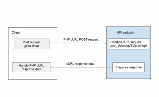
The cURL is a way of remote accessing the API endpoint over the network. The below code will save you time to achieve posting JSON data via PHP cURL.
Example: PHP cURL POST by Sending JSON Data
It prepares the JSON from an input array and bundles it to the PHP cURL post.
It uses PHP json_encode function to get the encoded request parameters. Then, it uses the CURLOPT_POSTFIELDS option to bundle the JSON data to be posted.
curl-post-json.php
<?php
// URL of the API that is to be invoked and data POSTed
$url = 'https://example.com/api-to-post'; // request data that is going to be sent as POST to API
$data = array( "animal" => "Lion", "type" => "Wild", "name" => "Simba", "zoo" => array( "address1" => "5333 Zoo", "city" => "Los Angeles", "state" => "CA", "country" => "USA", "zipcode" => "90027" )
); // encoding the request data as JSON which will be sent in POST
$encodedData = json_encode($data); // initiate curl with the url to send request
$curl = curl_init($url); // return CURL response
curl_setopt($curl, CURLOPT_RETURNTRANSFER, true); // Send request data using POST method
curl_setopt($curl, CURLOPT_CUSTOMREQUEST, "POST"); // Data conent-type is sent as JSON
curl_setopt($curl, CURLOPT_HTTPHEADER, array( 'Content-Type:application/json'
));
curl_setopt($curl, CURLOPT_POST, true); // Curl POST the JSON data to send the request
curl_setopt($curl, CURLOPT_POSTFIELDS, $encodedData); // execute the curl POST request and send data
$result = curl_exec($curl);
curl_close($curl); // if required print the curl response
print $result;
?>
The above code is one part of the API request-response cycle. If the endpoint belongs to some third-party API, this code is enough to complete this example.
But, if the API is in the intra-system (custom API created for the application itself), then, the posted data has to be handled.
How to get the JSON data in the endpoint
This is to handle the JSON data posted via PHP cURL in the API endpoint.
<?php
// use the following code snippet to receive
// JSON POST data
// json_decode converts the JSON string to JSON object
$data = json_decode(file_get_contents('php://input'), true);
print_r($data);
echo $data;
?>
The json_encode function also allows setting the allowed nesting limit of the input JSON. The default limit is 512.
If the posted JSON data is exceeding the nesting limit, then the API endpoint will be failed to get the post data.
Other modes of posting data to a cURL request
In a previous tutorial, we have seen many examples of sending requests with PHP cURL POST.
This program sets the content type “application/json” in the CURLOPT_HTTPHEADER. There are other modes of posting data via PHP cURL.
multipart/form-data – to send an array of post data to the endpoint/
application/x-www-form-urlencoded – to send a URL-encoded string of form data.
Note: PHP http_build_query() can output the URL encoded string of an array. Download
Do you need to create a function that returns a string but you don’t know how? No worries, in sixty seconds, you’ll know! Go!
A Python function can return any object such as a string. To return a string, create the string object within the function body, assign it to a variable my_string, and return it to the caller of the function using the keyword operation return my_string. Or simply create the string within the return expression like so: return "hello world"
def f(): return 'hello world' f()
# hello world
Create String in Function Body
Let’s have a look at another example:
The following code creates a function create_string() that iterates over all numbers 0, 1, 2, …, 9, appends them to the string my_string, and returns the string to the caller of the function:
def create_string(): ''' Function to return string ''' my_string = '' for i in range(10): my_string += str(i) return my_string s = create_string()
print(s)
# 0123456789
Note that you store the resulting string in the variable s. The local variable my_string that you created within the function body is only visible within the function but not outside of it.
So, if you try to access the name my_string, Python will raise a NameError:
>>> print(my_string)
Traceback (most recent call last): File "<pyshell#1>", line 1, in <module> print(my_string)
NameError: name 'my_string' is not defined
To fix this, simply assign the return value of the function — a string — to a new variable and access the content of this new variable:
>>> s = create_string()
>>> print(s)
0123456789
There are many other ways to return a string in Python.
Return String With List Comprehension
For example, you can use a list comprehension in combination with the string.join() method instead that is much more concise than the previous code—but creates the same string of digits:
def create_string(): ''' Function to return string ''' return ''.join([str(i) for i in range(10)]) s = create_string()
print(s)
# 0123456789
For a quick recap on list comprehension, feel free to scroll down to the end of this article.
You can also add some separator strings like so:
def create_string(): ''' Function to return string ''' return ' xxx '.join([str(i) for i in range(10)]) s = create_string()
print(s)
# 0 xxx 1 xxx 2 xxx 3 xxx 4 xxx 5 xxx 6 xxx 7 xxx 8 xxx 9
def create_string(): ''' Function to return string ''' return 'ho' * 10 s = create_string()
print(s)
# hohohohohohohohohoho
String Concatenation of Function Arguments
Here’s an example of string concatenation that appends all arguments to a given string and returns the result from the function:
def create_string(a, b, c): ''' Function to return string ''' return 'My String: ' + a + b + c s = create_string('python ', 'is ', 'great')
print(s)
# My String: python is great
Concatenate Arbitrary String Arguments and Return String Result
You can also use dynamic argument lists to be able to add an arbitrary number of string arguments and concatenate all of them:
def create_string(*args): ''' Function to return string ''' return ' '.join(str(x) for x in args) print(create_string('python', 'is', 'great'))
# python is great print(create_string(42, 41, 40, 41, 42, 9999, 'hi'))
# 42 41 40 41 42 9999 hi
Background List Comprehension
Knowledge: List comprehension is a very useful Python feature that allows you to dynamically create a list by using the syntax [expression context]. You iterate over all elements in a given context “for i in range(10)“, and apply a certain expression, e.g., the identity expression i, before adding the resulting values to the newly-created list.
In case you need to learn more about list comprehension, feel free to check out my explainer video:
Programmer Humor
Q: How do you tell an introverted computer scientist from an extroverted computer scientist? A: An extroverted computer scientist looks at your shoes when he talks to you.
Although Neural Networks do a tremendous job learning rules in tabular, structured data, it leaves a great deal to be desired in terms of ‘unstructured’ data. And there we come to a new concept: Recurrent Neural Networks.
Recurrent Neural Network
A Recurrent Neural Network is to a Feedforward Neural Network as a single object is to a list: it may be thought as a set of interrelated feedforward networks, or a looped network.
It is specialized in picking up and highlighting the main characteristics of your data (more on that in Andrej Karpathy’s Blog). They are often followed by a Feed Forward (Dense) Layer which will weigh the output.
Long Short-Term Memory
Long Short-Term Memory (LSTM) clusters have the extra special ability to deal with time (more on it can be found in Colah’s article).
As the term memory suggests, its greatest promise is to understand correlations between past and present events. In particular, they fit naturally in time series forecasts.
Here we aim at a hands-on introduction to several LSTM-based architectures (and more is to come ).
Article Overview
We use Bitcoin daily closing price as a case study. Specifically, we use the Bitcoin price and sentiment analysis we have gathered in a previous article. We use TensorFlow‘s Keras API for the implementation.
In this article will aim at the following architectures:
‘Vanilla’ LSTM
Stacked LSTM
Bidirectional LSTM
Encoder-Decoder LSTM-LSTM
Encoder-Decoder CNN-LSTM
The last one being the more convoluted (pun intended).
There is one main issue dealing with time series, which is the implementation of the problem. Are common situation both having only the historical target value alone (univariate problem) or together with other information (multivariate problem).
Moreover, you might be interested in one-step prediction or a multi-step prediction, i.e., predicting only the next day or, say, all days in the next week. Although it doesn’t sound so, you have to adjust your model to whatever situation you are facing.
Think of how you would deal with a multivariate multi-step problem: should you train a one-step model and forecast all features in order to feed your model to predict the following days? That would be a crazy!
Kaggle’s time series course does a good job introducing the several strategies present to deal with multi-step prediction. Fortunately, setting an LSTM network for a multi-step multivariate problem is as easy as setting it for a univariate one-step problem – you just need to change two numbers.
This is another advantage of Neural Networks, apart from its capacity of memory.
Of course, the architecture list above is not exhaustive. For instance, a new Attention layer was recently introduced, which has been working wonders. We shall come back to it in a next article, where we will walk through a hybrid Attention-CLX model.
Disclaimer: This article is a programming/data analysis tutorial only and is not intended to be any kind of investment advice.
How to Prepare the Data for LSTM?
We will use two sources of data, both explicit in our previous article: the SentiCrypt‘s Bitcoin sentiment analysis and Bitcoin’s daily closing price (by following the steps in the previous article, you can do it differently, using a minute-base data, for example).
Let us load the already-saved sentiment analysis and download the Bitcoin price:
import pandas as pd
import yfinance as yf sentic = pd.read_csv('sentic.csv', index_col=0, parse_dates=True)
sentic.index.freq='D' btc = yf.download('BTC-USD', start='2020-02-14', end='2022-09-23', period='1d')[['Close']]
btc.columns = ['btc'] data = pd.concat([sentic,btc], axis=1) data
The LSTM layer expects a 3D array as input whose shape represents:
(data_size, timesteps, number_of_features).
Meaning, the first and last elements are the number of rows and columns from the input data, respectively. The timestep argument is the size of the time chunk you want your LSTM to process at a time. This will be the time frame the LSTM will look for relations between past and present. It is essentially the size of its (long short-term) memory.
To decide how many time-steps, we recall our first time series article where we explored partial auto-correlations of Bitcoin price’s lags.
from statsmodels.graphics.tsaplots import plot_pacf
import matplotlib.pyplot as plt plot_pacf(data.btc, lags=20)
plt.show()
If you were there, in the first article, with me, you might remember our curious 10-lags correlation. Here we use this magic number and feed the model with a 10 days frame and to make a 5 days prediction. I found the results with 10 days better than for 6 or 20 days (for most cases – see below for more about this). We also assume we have today’s data and try to forecast the next 5 days.
An easy way to accomplish the reshaping of the data is through (a slight modification) of our make_lags function together with NumPy’s reshape() method.
So, instead of a Series, we will take a DataFrame as input and will output a concatenation of the original frame with its respective lags. We use negative lags to prepare the target DataFrame. We will ignore observations with the produced NaN values and will use the align method to align their indexes.
def make_lags(df, n_lags=1, lead_time=1): """ Compute lags of a pandas.DataFrame from lead_time to lead_time + n_lags. Alternatively, a list can be passed as n_lags. Returns a pd.DataFrame resulting from the concatenation of df's shifts. """ if isinstance(n_lags,int): lag_list = range(lead_time, n_lags+lead_time) else: lag_list = n_lags lags=list() for i in lag_list: df_lag = df.shift(i) if i!=0: df_lag.columns = [f'{col}_lag_{i}' for col in df.columns] lags.append(df_lag) return pd.concat(lags, axis=1) X = make_lags(data, n_lags=20, lead_time=0).dropna()
y = make_lags(data[['btc']], n_lags=range(-5,0)).dropna() X, y = X.align(y, join='inner', axis=0)
Next, we train-test split the data with sklearn, taking 10% as test size. As usual for time series, we include shuffle=False as a parameter.
from sklearn.model_selection import train_test_split X_train, X_val, y_train, y_val = train_test_split(X, y, test_size=.1, shuffle=False)
Before proceeding, it is good practice to normalize the data before feeding it into a Neural Network. We do it now, before things get 3D.
Finally, we use NumPy to reshape everything to 3D arrays. Observe that there is not such a thing as a 3D pd.DataFrame.
import numpy as np def add_dim(df, timesteps=5): """ Transforms a pd.DataFrame into a 3D np.array with shape (n_samples, timesteps, n_features) """ df = np.array(df) array_3d = df.reshape(df.shape[0],timesteps ,df.shape[1]//timesteps) return array_3d X_train, X_val = map(add_dim, [X_train, X_val], [timesteps]*2)
Of course, you can always prepare a function to do everything in one shot:
def prepare_data(df, target_name, n_lags, n_steps, lead_time, test_size, normalize=True): ''' Prepare data for LSTM. ''' if isinstance(n_steps,int): n_steps = range(1,n_steps+1) n_steps = [-x for x in list(n_steps)] X = make_lags(df, n_lags=n_lags, lead_time=lead_time).dropna() y = make_lags(df[[target_name]], n_lags=n_steps).dropna() X, y = X.align(y, join='inner', axis=0) from sklearn.model_selection import train_test_split X_train, X_val, y_train, y_val = train_test_split(X, y, test_size=test_size, shuffle=False) if normalize: from sklearn.preprocessing import MinMaxScaler mms = MinMaxScaler().fit(X_train) X_train, X_val = mms.transform(X_train), mms.transform(X_val) if isinstance(n_lags,int): timesteps = n_lags else: timesteps = len(n_lags) return add_dim(X_train,timesteps), add_dim(X_val,timesteps), y_train, y_val
Note that one should give positive values to n_steps to have the right negative shifts. Fortunately, y_train, y_val are not reshaped, which makes life easier when comparing predictions with reality.
All set, let’s start with the most basic Vanilla model.
Side note: We are keeping things simple here, but in a future post, we will prepare our own batches and explore better the stateful parameter of an LSTM layer. More on its input and output can be found in Mohammad’s Git.
How to Implement Vanilla LSTM with Keras?
A model is called Vanilla when it has no additional structure apart from the output layer.
To implement it we add an LSTM and a Dense layer. We must pass the number of units of each and the input shape for the LSTM layer.
The input shape is exactly (n_timesteps, n_features) which can be inferred from X_train.shape. The number of units for the LSTM layer is a hyperparameter and shall be tuned, for the Dense layer it is the number of outputs we want. Therefore 5.
Next follows a hypertuning-friendly code, specifying the main parameters in advance.
The model_paramsdictionary will be useful for including additional parameters to the compile method, such as an EarlyStopping callback.
We also write a function that fits the model, plot and assess predictions. The present code does not output anything, so, feel free to change it in order to do so. We fix the optimizer as Adam and the loss metric as Mean Squared Error.
def fit_model(model, learning_rate=0.001, time_distributed=False, epochs=epochs, batch_size=batch_size, verbose=verbose): y_ind = y_val.index if time_distributed: y_train_0 = y_train.to_numpy().reshape((y_train.shape[0], y_train.shape[1],1)) y_val_0 = y_val.to_numpy().reshape((y_val.shape[0], y_val.shape[1],1)) else: y_train_0 = y_train y_val_0 = y_val # fit network from keras.optimizers import Adam adam = Adam(learning_rate=learning_rate) model.compile(loss='mse', optimizer='adam') history = model.fit(X_train, y_train_0, epochs=epochs, batch_size=batch_size, verbose=verbose, **model_params, validation_data=(X_val, y_val_0), shuffle=False) # make a prediction if time_distributed: predictions = model.predict(X_val)[:,:,0] else: predictions = model.predict(X_val) yhat = pd.DataFrame(predictions, index=y_ind, columns=[f'pred_lag_{i}' for i in range(-n_steps,0)]) yhat_shifted = pd.concat([yhat.iloc[:,i].shift(-n_steps+i) for i in range(len(yhat.columns))], axis=1) # calculate RMSE from sklearn.metrics import mean_squared_error, r2_score rmse = np.sqrt(mean_squared_error(y_val, yhat)) import matplotlib.pyplot as plt fig, (ax1,ax2) = plt.subplots(2,1,figsize=(14,14)) y_val.iloc[:,0].plot(ax=ax2,legend=True) yhat_shifted.plot(ax=ax2) ax2.set_title('Prediction comparison') ax2.annotate(f'RMSE: {rmse:.5f} \n R2 score: {r2_score(yhat,y_val):.5f}', xy=(.68,.93), xycoords='axes fraction') ax1.plot(history.history['loss'], label='train') ax1.plot(history.history['val_loss'], label='test') ax1.legend() plt.show()
The time_distributed parameter will be used in the last two architectures.
I opted to set a manual learning_rate since once the Stacked LSTM’s output was an array of NaNs. After figuring out that the gradient descent was not converging, that was fixed by decreasing Adam’s learning rate.
Use verbose=1 as a global parameter to debug your network.
Without further ado:
fit_model(vanilla)
The performance is comparable to our XGBoost 1-day prediction in the last article:
Moreover, we are predicting 5 days, not only one, making the r2 score more impressive.
What bothers me, on the other hand, is the fact the predictions for all five days look identical. It requires further analysis to understand why that is happening, which we will not do here.
How to Build a Stacked LSTM?
We also can queue two LSTM layers.
To this aim, we need to be careful to give a 3D input to the second LSTM layer and that is the role the parameter return_sequences plays. We gain a slight increase in the training score in this case.
In general, any RNN within minimal requirements can be made bidirectional through Keras’ Bidirectional layer. It stacks two copies of your RNN layer, making one backward.
You can either specify the backward_layer as a second RNN layer or just wrap a single one, which will make the Bidirectional instance use a copy as the backward model. An implementation can be found below.
An Encoder-Decoder structure is designed in a way you have one network dedicated to feature selection and a second one to the actual forecast. The architectures used can be of different types; even of recurrent-non recurrent pairs are allowed.
Here we explore two pairs: LSTM-LSTM and CNN-LSTM.
Compared to the previous presented architectures, the main difference is the inclusion of the RepeatVector layer and the wrapper TimeDistributed.
Although the RepeatVector is smoothly included, the TimeDistributed layer needs some care. It wraps a layer object and has the duty to apply a copy of each to each temporal slice imputed into it. It considers the .shape[1] of the first input as the temporal dimension (our prepare_data is in accordance to that).
Moreover, one has to watch out since it outputs a 3D array, in particular our model will output 3D predictions.
For this reason, we have to feed the model with reshaped y_val, y_train so that the loss functions can be computed. Fortunately, we already included the time_distributed parameter in the fit_model to deal with the reshaping.
We also increase the number of Epochs since these networks seem to take longer to find a minimum. We include an EarlyStopping though. It already gives an astonishing score!
This is the first time the steps outputs are visibly different from each other.
Nevertheless, it seems to be following some trend. In theory, the NN should be so powerful that it can capture trends as well. However, in practice detrending often gives better results. Nevertheless, 0.82 is a massive increase from our 0.32 XGBoost.
Encoder-Decoder CNN-LSTM Network
The last architecture we present is the CNN-LSTM one.
Here a Convolutional Neural Network is used as a feature selector, being well-known to perform well in this role for photos and videos.
The main reason they are so useful in this case is mathematical: the convolutional part of CNN’s name refers to the convolution operationin mathematics, which is used to emphasize translation-invariant features.
That makes complete sense when you have a photo, since you want your mobile phone to recoginze Toto as a dog, independent if it is in the lower-left corner or in the upper-center of the picture (of course your dog’s name is Toto, right?). You may recognize the CNN action as the smoothed lines in the graph.
For the sake of completion, we tweaked the code around a bit.
Do you remember the seemly significant correlation popped up in the 20-days lags? Well, increasing from 10 to 20 timesteps actually increases the R2 score in the last model:
Funnily enough, it increases even more if you use unnormalized data, making a stellar ~.94 score!
The last thing worth mentioning is the choice of the activation function. If you got the Warning below and wonder why, the Keras’ LSTM documentation provides an answer.
WARNING: tensorflow:Layer lstm_70 will not use cuDNN kernels since it doesn’t meet the criteria. It will use a generic GPU kernel as fallback when running on GPU.
(No, I did not loaded 70 LSTM layers. I loaded around 210 )
The documentation says:
“The requirements to use the cuDNN implementation are:
activation == tanh
recurrent_activation == sigmoid
recurrent_dropout == 0
unroll is False
use_bias is True
Inputs, if use masking, are strictly right-padded.
Eager execution is enabled in the outermost context.”
Changing the activation to ‘tanh‘ is enough in our case to use cuDNN, and they are incredibly faster! However tanh fits poorly into our problem:
(You saw it right, the learning rate is 1000x larger than the default. Otherwise the loss curve does not even change.)
Main Takeaways
There are a few points we have to keep in mind about LSTM:
The shape of their input
What are time steps
The shape of the layer’s output, especially when using return_sequences
Hyperparameters tunning is worth your time. For instance, the activation functions relu and tanh have their own pros and cons.
There are different architectures to play with (and many more to come – we will deal with Attention blocks and Multi-headed networks soon). Consider using them. I’ve become specially inclined towards the Encoder-Decoders
Do you want to learn Solidity and create your own dApps and smart contracts? This free online course gives you a comprehensive overview that is aimed to be more accessible than the Solidity documentation but still complete and descriptive.
Multimodal Learning: Each tutorial comes with a tutorial video that helps you grasp the concepts in a more interactive manner.
Google Sheets API provides services of to read and write a Google spreadsheet document.
This tutorial is for reading data from Google sheets and displaying them in the UI with JavaScript. Only JavaScript is used without any plugins or dependencies.
Steps to access Google Sheets
It requires the following steps to achieve this.
Get OAuth Credentials and API keys and configure them into an application.
Authenticate and Authorise the app to allow accessing Google sheets.
We have also seen how to upload to Google Drive using PHP. It doesn’t need API Key. Instead, it does token-based authentication to get API access.
Step 1: Get OAuth Credentials and API keys and configure them into an application
In this step, it needs to create a developer’s web client app to get the client id and the API keys. For that, it requires the following setting should be enabled with the developer’s dashboard.
Login to the Google Developers console and create a web client.
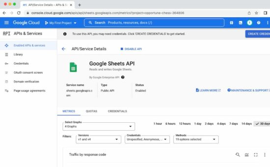
Enable Google Sheets API from the gallery of Google APIs.
Configure OAuth content screen to set the app details
Click OAuth credentials and get the app client id and secret key.
Set the scope on which the program going to access the spreadsheet.
Get the API key to authenticate and authorize the app to access the Google Spreadsheet API service.
Note: The secret key will be used for server-side implementation, but not in this JavaScript example.
Required scope to access the spreadsheet data
The following scopes should be selected to read the Google Spreadsheets via a program.
…auth/spreadsheets – to read, edit, create and delete Spreadsheets.
…auth/spreadsheets.readonly – to read Spreadsheets.
…auth/drive – to read, edit, create and delete Drive files.
…auth/drive.readonly – to read Drive files
…auth/drive.file – to read, edit, create and delete a specific Drive files belongs to the app gets authorized.
Step 2: Authenticate and Authorise the app to allow accessing Google sheets
Authorization is the process of the client signing into the Google API to access its services.
On clicking an “Authorize” button, it calls authorizeGoogleAccess() function created for this example.
This function shows a content screen for the end user to allow access. Then, it receives the access token in a callback handler defined in this function.
Step 3: Read spreadsheet data and store it in an array
Once access is permitted, the callback will invoke the script to access an existing Google spreadsheet.
The listMajors() function specifies a particular spreadsheet id to be accessed. This function uses JavaScript gapi instance to get the spreadsheet data.
Step 4: Parse response data and display them on the UI
After getting the response data from the API endpoint, this script parses the resultant object array.
It prepares the output HTML with the spreadsheet data and displays them to the target element.
If anything strange with the response, it shows the “No records found” message in the browser.
A complete code: Accessing Google Spreadsheets via JavaScript
The following script contains the HTML to show either “Authorize” or the two “Refresh” and “Signout” buttons. Those buttons’ display mode is based on the state of authorization to access the Google Spreadsheet API.
The example code includes the JavaScript library to make use of the required Google API services.
The JavaScript has the configuration to pin the API key and OAuth client id in a right place. This configuration is used to proceed with the steps 2, 3 and 4 we have seen above.
<!DOCTYPE html>
<html>
<head>
<title>Google Sheets JavaScript API Spreadsheet Tutorial</title>
<link rel='stylesheet' href='style.css' type='text/css' />
<link rel='stylesheet' href='form.css' type='text/css' />
</head>
<body> <div class="phppot-container"> <h1>Google Sheets JavaScript API Spreadsheet Tutorial</h1> <p>This tutorial is to help you learn on how to read Google Sheets (spreadsheet) using JavaScript Google API.</p> <button id="authorize_btn" onclick="authorizeGoogleAccess()">Authorize Google Sheets Access</button> <button id="signout_btn" onclick="signoutGoogle()">Sign Out</button> <pre id="content"></pre> </div> <script async defer src="https://apis.google.com/js/api.js" onload="gapiLoaded()"></script> <script async defer src="https://accounts.google.com/gsi/client" onload="gisLoaded()"></script>
</body>
</html>
// You should set your Google client ID and Google API key
const GOOGLE_CLIENT_ID = '';
const GOOGLE_API_KEY = '';
// const DISCOVERY_DOC = 'https://sheets.googleapis.com/$discovery/rest?version=v4'; // Authorization scope should be declared for spreadsheet handing
// multiple scope can he included separated by space
const SCOPES = 'https://www.googleapis.com/auth/spreadsheets.readonly'; let tokenClient;
let gapiInited = false;
let gisInited = false;
document.getElementById('authorize_btn').style.visibility = 'hidden';
document.getElementById('signout_btn').style.visibility = 'hidden'; /** * Callback after api.js is loaded. */
function gapiLoaded() { gapi.load('client', intializeGapiClient);
} /** * Callback after the Google API client is loaded. Loads the * discovery doc to initialize the API. */
async function intializeGapiClient() { await gapi.client.init({ apiKey: GOOGLE_API_KEY, discoveryDocs: [DISCOVERY_DOC], }); gapiInited = true; maybeEnableButtons();
} /** * Callback after Google Identity Services are loaded. */
function gisLoaded() { tokenClient = google.accounts.oauth2.initTokenClient({ client_id: GOOGLE_CLIENT_ID, scope: SCOPES, callback: '', // defined later }); gisInited = true; maybeEnableButtons();
} /** * Enables user interaction after all libraries are loaded. */
function maybeEnableButtons() { if (gapiInited && gisInited) { document.getElementById('authorize_btn').style.visibility = 'visible'; }
} /** * Sign in the user upon button click. */
function authorizeGoogleAccess() { tokenClient.callback = async (resp) => { if (resp.error !== undefined) { throw (resp); } document.getElementById('signout_btn').style.visibility = 'visible'; document.getElementById('authorize_btn').innerText = 'Refresh'; await listMajors(); }; if (gapi.client.getToken() === null) { // Prompt the user to select a Google Account and ask for consent to share their data // when establishing a new session. tokenClient.requestAccessToken({ prompt: 'consent' }); } else { // Skip display of account chooser and consent dialog for an existing session. tokenClient.requestAccessToken({ prompt: '' }); }
} /** * Sign out the user upon button click. */
function signoutGoogle() { const token = gapi.client.getToken(); if (token !== null) { google.accounts.oauth2.revoke(token.access_token); gapi.client.setToken(''); document.getElementById('content').innerText = ''; document.getElementById('authorize_btn').innerText = 'Authorize'; document.getElementById('signout_btn').style.visibility = 'hidden'; }
} /** * Print the names and majors of students in a sample spreadsheet: * https://docs.google.com/spreadsheets/d/1aSSi9jk2gBEHXOZNg7AV7bJj0muFNyPLYwh2GXThvas/edit */
async function listMajors() { let response; try { // Fetch first 10 files response = await gapi.client.sheets.spreadsheets.values.get({ spreadsheetId: '', range: 'Sheet1!A2:D', }); } catch (err) { document.getElementById('content').innerText = err.message; return; } const range = response.result; if (!range || !range.values || range.values.length == 0) { document.getElementById('content').innerText = 'No values found.'; return; } const output = range.values.reduce( (str, row) => `${str}${row[0]}, ${row[2]}\n`, 'Birds, Insects:\n'); document.getElementById('content').innerText = output;
}
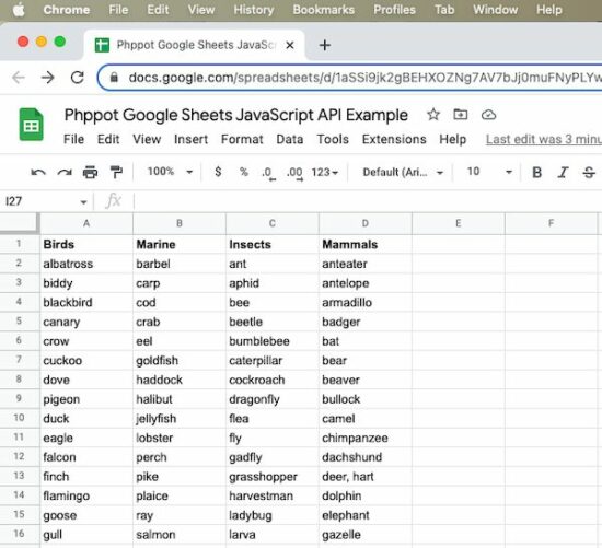
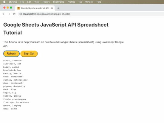
Source and output of this example
The spreadsheet shown in this screenshot is the source of this program to access its data.
The JavaScript example reads the spreadsheet and displays the Birds and the Insects column data in the UI.


 Here you will find additional examples of Plotly Dash components, layouts and style. To learn more about making dashboards with Plotly Dash, and how to buy your copy of

 Recommended Resource: For more information about styling your app with a Boostrap theme, see


 GitHub:
  Dash Forum:
  YouTube CharmingData:
  Python + Crypto Email Academy:

 Full Guide:


 ).
). 
 Disclaimer: This article is a programming/data analysis tutorial only and is not intended to be any kind of investment advice.


 WARNING:
  )
)