Example 1 – Disabling cut, copy, paste and mouse right-click events
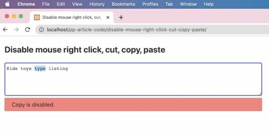
This JavaScript disables the cut, copy, paste and right-click on a textarea content.
It defines a callback invoked on document ready event. It uses jQuery.
In this callback, it listens to the cut, copy, paste and the mouse right-click action requests.
When these requests are raised this script prevents the default behavior. Hence, it stops the expected action based on the cut, copy, and other requests mentioned above.
This example is a thin version of the above. It also uses the jQuery library to disable the cut, copy paste and right-click events.
This binds all the events to be disabled. It has a single-line code instead of creating exclusive listeners for each event.
This method has a slight disadvantage. That is, it shows a generic message while stopping any one of the cut, copy, paste and right-click events.
In the first method, the acknowledgment message is too specific. That message gives more clarity on what is triggered and what is disabled and prevented.
But, the advantage of the below example is that it is too thin to have it as a client-side feature in our application.
$(document).ready(function() { $('textarea').bind('cut copy paste contextmenu', function(e) { e.preventDefault(); $("#phppot-message").text('The Cut copy paste and the mouse right-click are disabled.'); $("#phppot-message").show(); });
});
Example 3 – For JavaScript lovers
Do you want a pure JavaScript solution for this example? The below script achieves this to disable cut, copy, paste and right-click.
It has no jQuery or any other client-side framework or libraries. I believe that the frameworks are for achieving a volume of effects, utils and more.
If the application is going to have thin requirements, then no need for any framework.
HTML with onCut, onCopy, onPaste and onContextMenu attributes
The Textarea field in the below HTML has the following callback attributes.
onCut
OnCopy
onPaste
onContextMenu
In these event occurrences, it calls the disableAction(). It sends the event object and a string to specify the event occurred.
JavaScript function called on cut, copy, paste and on right click
In the JavaScript code, it reads the event type and disables it.
The event.preventDefault() is the common step in all the examples to disable the cut, copy, paste and right click.
function disableAction(event, action) { event.preventDefault(); document.getElementById("phppot-message").innerText = action + ' is disabled.'; document.getElementById("phppot-message").style.display = 'block';
}
Disclaimer
The keyboard or mouse event callbacks like onMouseDown() or onKeyDown lags in performance. Also, it has its disadvantages. Some of them are listed below.
The keys can be configured and customized. So, event handling with respect to the keycode is not dependable.
On clicking the mouse right, it displays the menu before the onMouseDown() gets and checks the key code. So, disabling mouse-right-click is failed by using onMouseDown() callback.
Above all, an user can easily disable JavaScript in his browser and use the website.
To append a row (=dictionary) to an existing CSV, open the file object in append mode using open('my_file.csv', 'a', newline=''). Then create a csv.DictWriter() to append a dict row using DictWriter.writerow(my_dict).
Given the following file 'my_file.csv':
You can append a row (dict) to the CSV file via this code snippet:
import csv # Create the dictionary (=row)
row = {'A':'Y1', 'B':'Y2', 'C':'Y3'} # Open the CSV file in "append" mode
with open('my_file.csv', 'a', newline='') as f: # Create a dictionary writer with the dict keys as column fieldnames writer = csv.DictWriter(f, fieldnames=row.keys()) # Append single row to CSV writer.writerow(row)
After running the code in the same folder as your original 'my_file.csv', you’ll see the following result:
Append Multiple Rows to CSV
Given the following CSV file:
To add multiple rows (i.e., dicts) to an old existing CSV file, iterate over the rows and write each row by calling csv.DictWriter.writerow(row) on the initially created DictWriter object.
Here’s an example (major changes highlighted):
import csv # Create the dictionary (=row)
rows = [{'A':'Z1', 'B':'Z2', 'C':'Z3'}, {'A':'ZZ1', 'B':'ZZ2', 'C':'ZZ3'}, {'A':'ZZZ1', 'B':'ZZZ2', 'C':'ZZZ3'}] # Open the CSV file in "append" mode
with open('my_file.csv', 'a', newline='') as f: # Create a dictionary writer with the dict keys as column fieldnames writer = csv.DictWriter(f, fieldnames=rows[0].keys()) # Append multiple rows to CSV for row in rows: writer.writerow(row)
The resulting CSV file has all three rows added to the first row:
Python Add Row to CSV Pandas
To add a row to an existing CSV using Pandas, you can set the write mode argument to append 'a' in the pandas DataFrame to_csv() method like so: df.to_csv('my_csv.csv', mode='a', header=False).
df.to_csv('my_csv.csv', mode='a', header=False)
For a full example, check out this code snippet:
import pandas as pd # Create the initial CSV data
rows = [{'A':'Z1', 'B':'Z2', 'C':'Z3'}, {'A':'ZZ1', 'B':'ZZ2', 'C':'ZZ3'}, {'A':'ZZZ1', 'B':'ZZZ2', 'C':'ZZZ3'}] # Create a DataFrame and write to CSV
df = pd.DataFrame(rows)
df.to_csv('my_file.csv', header=False, index=False) # Create another row and append row (as df) to existing CSV
row = [{'A':'X1', 'B':'X2', 'C':'X3'}]
df = pd.DataFrame(row)
df.to_csv('my_file.csv', mode='a', header=False, index=False)
The output file looks like this (new row highlighted):
Alternatively, you can open the file in append mode using normal open() function with the append 'a' argument and pass it into the pandas DataFrame to_csv() method.
Here’s an example snippet for copy&paste:
with open('my_csv.csv', 'a') as f: df.to_csv(f, header=False)
Question: How to convert a dictionary to a CSV in Python?
In Python, convert a dictionary to a CSV file using the DictWriter() method from the csv module. The csv.DictWriter() method allows you to insert a dictionary-formatted row (keys=column names; values=row elements) into the CSV file using its DictWriter.writerow() method.
You create a Pandas DataFrame—which is Python’s default representation of tabular data. Think of it as an Excel spreadsheet within your code (with rows and columns).
The DataFrame is a very powerful data structure that allows you to perform various methods. One of those is the to_csv() method that allows you to write its contents into a CSV file.
You set the index argument of the to_csv() method to False because Pandas, per default, adds integer row and column indices 0, 1, 2, …. Again, think of them as the row and column indices in your Excel spreadsheet. You don’t want them to appear in the CSV file so you set the arguments to False.
You set the and header argument to True because you want the dict keys to be used as headers of the CSV.
If you want to customize the CSV output, you’ve got a lot of special arguments to play with. Check out this Finxter Tutorial for a comprehensive list of all arguments.
In Python, convert a dictionary to a CSV file using the DictWriter() method from the csv module. The csv.DictWriter() method allows you to insert data into the CSV file using its DictWriter.writerow() method.
The following example writes the dictionary to a CSV using the keys as column names and the values as row values.
import csv data = {'A':'X1', 'B':'X2', 'C':'X3'} with open('my_file.csv', 'w', newline='') as f: writer = csv.DictWriter(f, fieldnames=data.keys()) writer.writeheader() writer.writerow(data)
The resulting file 'my_file.csv' looks like this:
The csv library may not yet installed on your machine. To check if it is installed, follow these instructions. If it is not installed, fix it by running pip install csv in your shell or terminal.
Method 3: Dict to CSV String (in Memory)
To convert a list of dicts to a CSV string in memory, i.e., returning a CSV string instead of writing in a CSV file, use the pandas.DataFrame.to_csv() function without file path argument. The return value is a CSV string representation of the dictionary.
We pass index=False because we don’t want an index 0, 1, 2 in front of each row.
Method 4: Dict to CSV Append Line
To append a dictionary to an existing CSV, you can open the file object in append mode using open('my_file.csv', 'a', newline='') and using the csv.DictWriter() to append a dict row using DictWriter.writerow(my_dict).
Given the following file 'my_file.csv':
You can append a row (dict) to the CSV file via this code snippet:
import csv row = {'A':'Y1', 'B':'Y2', 'C':'Y3'} with open('my_file.csv', 'a', newline='') as f: writer = csv.DictWriter(f, fieldnames=row.keys()) writer.writerow(row)
After running the code in the same folder as your original 'my_file.csv', you’ll see the following result:
Method 5: Dict to CSV Columns
To write a Python dictionary in a CSV file as a column, i.e., a single (key, value) pair per row, use the following three steps:
Open the file in writing mode and using the newline='' argument to prevent blank lines.
Create a CSV writer object.
Iterate over the (key, value) pairs of the dictionary using the dict.items() method.
Write one (key, value) tuple at a time by passing it in the writer.writerow() method.
Here’s the code example:
import csv data = {'A':42, 'B':41, 'C':40} with open('my_file.csv', 'w', newline='') as f: writer = csv.writer(f) for row in data.items(): writer.writerow(row)
Your output CSV file (column dict) looks like this:
Method 6: Dict to CSV with Header
Convert a Python dictionary to a CSV file with header using the csv.DictWriter(fileobject, fieldnames) method to create a writer object used for writing the header via writer.writeheader() without argument. This writes the list of column names passed as fieldnames, e.g., the dictionary keys obtained via dict.keys().
To write the rows, you can then call the DictWriter.writerow() method.
The following example writes the dictionary to a CSV using the keys as column names and the values as row values.
import csv data = {'A':'X1', 'B':'X2', 'C':'X3'} with open('my_file.csv', 'w', newline='') as f: writer = csv.DictWriter(f, fieldnames=data.keys()) writer.writeheader() writer.writerow(data)
The resulting file 'my_file.csv' looks like this:
Where to Go From Here
If you haven’t found your solution, yet, you may want to check out my in-depth guide on how to write a list of dicts to a CSV:
If you don’t want to import any library and still convert a list of dicts into a CSV file, you can use standard Python implementation as well: it’s not complicated and very efficient.
This method is best if you won’t or cannot use external dependencies.
Open the file f in writing mode using the standard open() function.
Write the first dictionary’s keys in the file using the one-liner expression f.write(','.join(salary[0].keys())).
Iterate over the list of dicts and write the values in the CSV using the expression f.write(','.join(str(x) for x in row.values())).
Here’s the concrete code example:
salary = [{'Name':'Alice', 'Job':'Data Scientist', 'Salary':122000}, {'Name':'Bob', 'Job':'Engineer', 'Salary':77000}, {'Name':'Carl', 'Job':'Manager', 'Salary':119000}] # Method 3
with open('my_file.csv','w') as f: f.write(','.join(salary[0].keys())) f.write('n') for row in salary: f.write(','.join(str(x) for x in row.values())) f.write('n')
In the code, you first open the file object f. Then you iterate over each row and each element in the row and write the element to the file—one by one. After each element, you place the comma to generate the CSV file format. After each row, you place the newline character 'n'.
Note: to get rid of the trailing comma, you can check if the element x is the last element in the row within the loop body and skip writing the comma if it is.
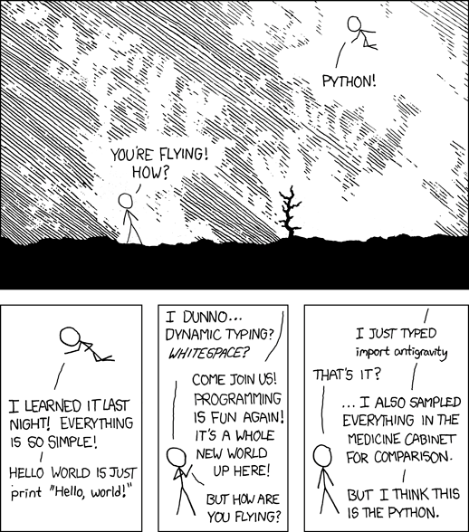
“I wrote 20 short programs in Python yesterday. It was wonderful. Perl, I’m leaving you.” — xkcd
Where to Go From Here?
Enough theory. Let’s get some practice!
Coders get paid six figures and more because they can solve problems more effectively using machine intelligence and automation.
To become more successful in coding, solve more real problems for real people. That’s how you polish the skills you really need in practice. After all, what’s the use of learning theory that nobody ever needs?
You build high-value coding skills by working on practical coding projects!
Do you want to stop learning with toy projects and focus on practical code projects that earn you money and solve real problems for people?
If your answer is YES!, consider becoming a Python freelance developer! It’s the best way of approaching the task of improving your Python skills—even if you are a complete beginner.
If you just want to learn about the freelancing opportunity, feel free to watch my free webinar “How to Build Your High-Income Skill Python” and learn how I grew my coding business online and how you can, too—from the comfort of your own home.
Artificial neural networks have become a powerful tool providing many benefits in our modern world. They are used to filter out spam, to perform voice recognition, and are even being developed to drive cars, among many other things.
As remarkable as these tools are, they are readily within the grasp of almost anyone. If you have technical interest and have some experience with computer programming you can build your own neural networks.
But before you learn the hands-on details of building neural networks you should learn some of the fundamentals of how they work. This article will cover one of those fundamentals – how neural networks learn.
Note: This article includes some algebra and calculus. If you’re not comfortable with algebra, you should still be able to understand the content from the graphs and descriptions. The calculus is not done in any detail. Again you should still be able to follow along from the descriptions. You will not learn the details of how the calculations are done. Instead, you will gain an intuitive understanding of what is going on.
Before learning this, you should be familiar with the basics of how neural networks are structured and how they operate. The article “The Magic of Neural Networks: History and Concepts” covers these basics. Still, we offer the following brief refresher.
Basic Fundamentals: How Neural Networks Work
Figure 1 shows an artificial neuron.
Figure 1: artificial neuron
Signals from other neurons come in through multiple inputs, each multiplied by its corresponding weight (Weights express the connection strengths between the neuron and each of its upstream neurons.).
A bias is input as well (bias expresses a neuron’s inherent activation, independent of its input from other neurons.). All these inputs add together, and the resulting total signal is then processed through the activation function (A sigmoid function is shown here.).
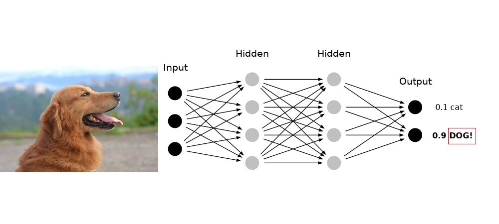
Figure 2: neural network classifying an image (Dog photo by Garfield Besa)
Figure 2 shows a network of these neurons. Signals are introduced on the input side, and they progress through the network, passing through neurons and along their connections, getting processed by the calculations described above. How the signals are processed, depends on the weights and biases among all the neurons.
The key takeaway is that it is the settings of the weights and biases that establish how the network as a whole computes. In other words, the learning and memory of the network is encoded by the weights and biases.
So how does one program these weights and biases?
They are set by training the network with samples and letting it learn by example. The details of how that is done is the subject of this article.
Overview of How Neural Networks Learn
As mentioned, a neural network’s learning and memory is encoded by the connection weights and biases of the neurons throughout the network.
These weights and biases are set by training the network on examples by following this six-step training procedure:
Provide a sample to the network.
Since the network is untrained, it will probably get the wrong answer.
Compute how far this answer is from the correct answer. This error is known as loss.
Calculate what changes in the weights and biases will make the loss smaller.
Make adjustments to those weights and biases as determined by those calculations.
Repeat this again and again with numerous samples until the network learns to answer the samples correctly.
Presenting Samples and Calculating Loss
Let’s review some of this in more detail while considering a use case.
Imagine we want to train a network to estimate crowd size.
To do this we must first train the network with a large set of images of crowds. For each image the number of people are counted. We then include labels indicating correct crowd size for each picture. This is known as a training set.
The pictures are submitted to the network, which then indicates its crowd estimate for each picture. Since the network is not trained, it surely gets the estimate wrong for each image.
For each image/label pair, the network calculates the loss for that sample.
Multiple possible choices can be used for calculating loss. One can choose any calculation that appropriately expresses how far the network’s answer is from the correct answer.
An appropriate choice for crowd-size loss estimate is the square error:
where:
Suppose we submit an image showing a crowd size of 500 people. Figure 3 shows how the error varies for crowd estimates around the true crowd size of 500 people.
Figure 3
If the Network guesses 350 people the loss is 22500. If the network guesses 600 people the loss is 10000.
Clearly, the loss is minimized when the network guesses the correct crowd size of 500 people.
But recall we said it is the weights and biases in the network that encode its learning and memory, so it is the weights and biases that determine if the network gets the right answer. So we need to adjust the weights and biases so that the network gets closer to the correct answer for this image.
In other words, we need to change the weights and biases to minimize the loss. To do that, we need to figure out how the loss varies when we vary the weights and biases.
Minimizing Loss: Calculus and the Derivative
So how do we calculate how loss changes when we vary weights and biases?
This is where calculus comes in.
(Don’t worry if you don’t know calculus, we’ll show you everything you need to know, and we’ll keep it intuitive.)
Calculus is all about determining how one variable is affected by changes in another variable.
(Strictly speaking there’s more to calculus than that, but this idea is one of the core ideas of calculus.)
The loss L depends on network output y, but y depends on input, and on weights w and biases b. So there is a somewhat long and complicated chain of dependencies we have to go through to figure out how L varies when w and b vary.
However, for the sake of learning, let’s instead start by just examing how L varies when y varies, since this is simpler and will help develop an intuition for calculus.
How L depends on y is somewhat easy – we saw the equation for it earlier, and we saw the graph of that equation in Figure 3. We can tell by looking at the graph that if the network guesses 350 then we need to increase the output y in order to reduce the loss, and that if the network guesses 600 then we need to decrease the output y in order to reduce the loss.
But with neural networks, we never have the luxury of being able to examine the graph of the loss to figure it out.
We can, however, use calculus to get our answer. To do this, we do what is called taking the derivative.
Here is the derivative of the equation for the graph in Figure 3 (note, we will not explain how this is calculated, that is the domain of a calculus course.):
This is typically referred to as “taking the derivative of L with respect to y”. You can read that dL/dy as saying “this is how L changes when y changes”. Now let’s calculate how L changes when y changes at the point y = 350:
So at y = 350, for every bit y increases, L decreases by 300. That implies that when we increase y the loss will decrease.
Now let’s calculate how L changes when y changes at the point y = 600:
So at y = 600, for every bit y increases, L increases by 200. Since we want to decrease L, that means we need to decrease y.
These calculations match what we concluded from looking at the graph.
You can also read dL/dy as saying “this is the slope of the graph”.
This makes sense: at point y = 350 the slope of the graph is -300 (sloping down steeply), while at point y = 600 the slope of the graph is 200 (sloping up, not quite so steeply).
So by using calculus and taking the derivative, we can figure out which way to change y to reduce the loss L, even when we can’t see the graph to figure it out.
Recall, however, that we want to figure out how to change the weights and biases to reduce the loss L. Also recall there is a chain of dependencies, of L depending on y, which itself depends on w and b (for several layers worth of w and b!), and on input.
So a full description could result in some rather complicated equations and some difficult derivatives. For those curious about the math details, the method for figuring out derivatives when there is such dependencies is called the chain rule.
Fortunately, with modern neural network software, the computer takes care of calculating derivatives and keeping track of and resolving the chains of dependencies in the derivatives. Just understand that, even if we can’t see its graph:
there is some relationship between the loss L and the weights w and biases b (a “graph”)
there is some set of weights and biases where the loss L is at a minimum for a given input
we can use calculus to figure out how to adjust the weights and biases to minimize loss
The Loss Surface and Gradient Descent
Let’s consider a very simple case where there are just two weights, w1 and w2, and no biases. The graph of L as a function of w1 and w2 might look like figure 4.
Figure 4: bowl-shaped error graph
In this example, with two independent weights, we end up with a bowl-shaped surface for the loss graph. In this case, the loss is minimized when w1 = 4 and w2 = 3. In the beginning, when the network is not yet trained the weights (initially set to small random numbers) are almost certainly not at the correct values for the loss to be at a minimum.
We still figure out which direction to change the weights to reduce the loss by taking the derivative.
Only this time, since there are two independent variables, we take the derivative with respect to each independently.
Important: The result is, for any given point on the loss surface, a direction (a vector, or an arrow) pointing in which direction the loss increases the fastest (“uphill”). This is known as the gradient (instead of derivative). Since we want to reduce loss, we move in the opposite direction, the negative of the gradient.
The larger point is we are still using calculus to figure out which direction to change weights to reduce loss. Repeatedly doing this moves the weights closer to the values which make the network give the correct answer for a given input. This is known as gradient descent.
However, most neural networks have many more than two weights, typically dozens for any given layer.
But the same ideas still apply: if we have a layer consisting of 16 weighted connections, the loss is a 16-dimensional surface! You can’t visualize it but it still exists mathematically, and the same principles apply!
You can still calculate the gradient, that is the derivative with respect to all 16 w’s, and figure out which direction to change the w’s to minimize the loss.
So how much do we adjust the weights and biases?
Typically they are adjusted just a small amount. This is because large adjustments can cause problems.
Refer to the loss surface shown in Figure 4. If too large a step is made, you could jump right across the loss surface bowl, even going so far as to make the loss worse!
The adjustment step size is known as the learning rate. Figuring out the best learning rate is one of the tricks to optimizing your network that a neural network engineer has to work out.
Backpropagation
Ultimately all of the weights and biases throughout the network have to be adjusted to minimize loss. This is done back from the loss, working back layer by layer to the beginning of the network, a process called backpropagation.
It has to be done this way because you can’t figure out how the first layer’s weights and biases affect loss until you know how the second layer’s weights and biases affect loss; you can’t tell how the second layer’s weights and biases effect loss until you know how the third layer’s weights and biases effect loss, and so on.
So calculations and adjustments are done starting with the last layer, then working back to the second to the last layer, and so on back to the first layer.
So that’s the core algorithm of training a neural network:
Present example image.
Calculate the loss.
Adjust the network weights and biases through backpropagation, calculating gradient descent, and making adjustments layer by layer.
Batch Size
However, recall that the objective of the training is to adjust the weights and biases for all of the images, not just one.
So how does one train the network, one image at a time, or using the entire set of all training images? Either choice is a possibility.
Ultimately the loss we want to minimize is the loss for the entire set of training samples, so a natural choice might be to run all samples through the network before making adjustments to the weights and biases. This is known as batch processing.
However performing so many calculations before making adjustments can be very demanding on computer resources and can slow the training process down.
How about adjusting weights and biases for each individual training sample? Optimum weights and biases will be different for each training sample, and this variation can introduce large randomness into the gradient descent. This is known as stochastic gradient descent.
To better understand the importance of this refer to the hypothetical loss curve in figure 5:
Figure 5: local and global minimum
Notice that there is more than one minimum: there is a local minimum at point B, which is not quite the lowest loss, and a global minimum at point A that is truly the minimum where the loss is lowest.
It is truly possible (even likely) to get loss curves like this, with multiple local minima, and it’s also possible for the network to get stuck in one of these local minima.
The randomness of single sample training can help knock the network out of a local minimum if it gets stuck in one, so there is some benefit to stochastic gradient descent.
However, the randomness can be so extreme that it can actually knock the network out of the true global minimum if it happens to reach it before a training cycle ends. This can slow the training as the network has to work back down to minimize the loss again.
So in practice, it turns out the best approach is to use minibatches. These are batch sizes of perhaps a few hundred samples that are run through the network, and then adjustments are made.
The network runs through mini batch after many batch until the entire set of training samples has been processed. This has enough randomness to it that it has the same benefit as stochastic gradient descent of pushing the network out of local minima, but not so much randomness that the loss can get worse.
Running through the entire set of training samples once is called an epoch.
Typically networks must run through many epochs to become fully trained. Also the ordering and grouping of training samples within and between batches is randomized from epoch to epoch. This is to avoid overfitting.
Overfitting is when the network performs successfully on the training samples, but fails on samples it has not seen before. This is like a person memorizing a set of samples, rather than generalizing characteritics from those samples so that it can be successful on new samples.
After training the network is then tested on a test set. This is a set of samples the network has not seen before. This allows one to assess how well the trained network performs. It checks to see how effective the network is on unknown samples, and checks to make sure overfitting has not occurred.
How Neural Networks Learn
So that is the full process of how neural networks learn:
Train the network by presenting it minibatches of samples from the training set.
The training algorithm calculates the loss for the minibatch.
The algorithm calculates the gradient of the loss.
The network adjusts weights and biases according to the gradient calculations, through the process of backpropagation and gradient descent.
Running this sequence through all training samples is called an epoch.
This is then repeated for multiple epochs, until the network is successfully trained on the training set.
Finally the network is tested on a test set to make sure it works successfully and does not suffer from overfitting.
We hope you have found this lesson on how neural networks learn informative.
Google reCaptcha V3 is the latest version provided with the highest security in comparison. Google contains different captcha services with reCaptcha V2. There are the (I am not a Robot) checkbox, invisible captcha and etc.
With the V3, Google guarantees zero friction while predicting the score for the website interactions. The score and the response report returned by the reCaptcha V3 is a very good security measure. It helps to take action accordingly to safeguard the website.
Like other Google reCaptcha concepts, the V3 also has more than one method to integrate the captcha challenge. Those are two as listed below.
Programmatic invocation of the challenge.
Automatic binding of the challenge with the form button.
This article explains to implement both methods by creating examples.
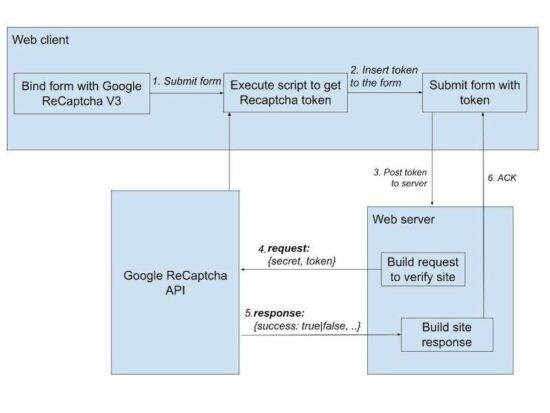
The below diagram will help to have a quick look at the Google reCaptcha V3 process flow. Continue reading to learn how to get the API keys and integrate reCaptcha for your website.
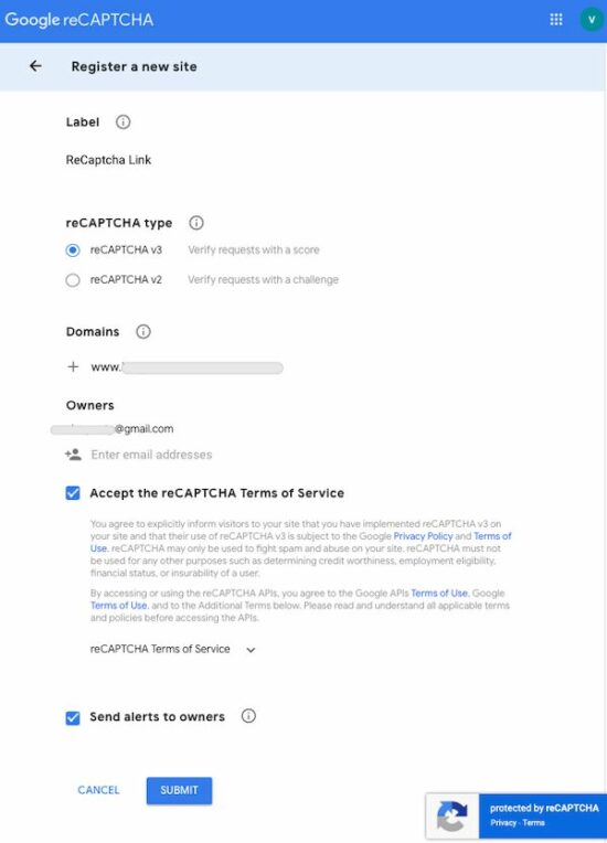
The below screenshot masked the data related to the domain and site owner details. Enter your site details in the place of the masked data.
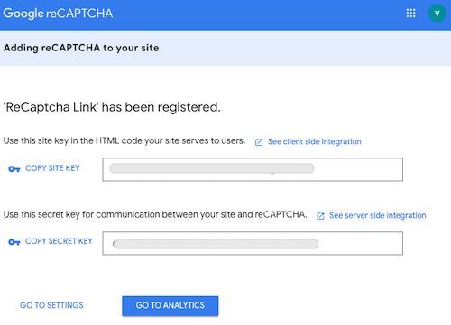
Step2: Copy the reCaptcha site key and the secret key.
Once registration is done, the reCaptcha V3 keys are displayed below. Copy these details and configure them into the website code.
The site key is used to render the Google reCaptcha on the client side. And, the secret key is used for server-side verification.
The following example contains an application configuration file for this. Continue reading to know how to configure.
About this example
This example renders the reCaptcha script and element in the landing UI. It has the configuration to make the website reCaptcha ready with the API keys.
It gets the token from the Google reCaptcha API and appends it to the form. On submit, the server-side PHP script receives the token to send the siteverify request to the API.
It integrates the Google reCaptcha V3 programmatic challenge in the root. If you want to implement the “automatic binding” method, then it is in a separate folder.
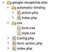
The below structure shows the reCaptcha example files order and location. It will be helpful to set up this code correctly in a development environment.
Application configuration file
It configures the Google reCaptcha V3 site and the secret keys used in the examples below.
The site key is used to render the Google recaptcha element on the client side. The secret key is used in the PHP files to build the site verification request parameters.
Method 1: Programatically invoking Google reCaptcha token via script
This method is used when the developer wants to have more programming control over the reCaptcha token.
During the explicit execution, it sets parameters to the request. These parameters can be returned with the Google reCaptcha V3 response. This will be helpful for additional verification.
HTML page renders form with reCaptcha JS
This landing page loads the JavaScript API while rendering the form UI. It uses the Google reCaptcha site key while loading the JavaScript.
// Execute Google reCaptcha v3 to get token function getToken(event) { event.preventDefault(); grecaptcha.ready(function() { grecaptcha.execute('<?php echo Config::GOOGLE_RECAPTCHA_SITE_KEY; ?>', { action: 'submit' }).then(function(token) { var button = document.createElement('input'); button.type = 'hidden'; button.name = 'recaptcha_token'; button.id = 'recaptcha_token'; button.value = token; var form = document.getElementById("frm"); form.appendChild(button); submitForm(); });; });
} // Submit reCaptcha token to the PHP
function submitForm() { const form = document.getElementById('frm'); const formData = new FormData(form); var xhttp = new XMLHttpRequest(); xhttp.open('POST', 'form-action.php', true); xhttp.send(formData); xhttp.onreadystatechange = function() { if (xhttp.readyState == 4 && xhttp.status == 200) { document.getElementById("ack-message").innerHTML = xhttp.responseText; document.getElementById('recaptcha_token').remove(); } }
}
Verify website interaction using Google reCaptcha V3 API
The form submits action calls this PHP script by sending the reCaptcha token. It builds the post parameters with the Google reCaptcha v3 secret key and token.
It returns the score about the interaction made on the website. This score will be between 0.0 (lower) and 1.1(higher) ranking. It helps to predict the necessary steps to make to protect the site.
Method 2: Automatic binding callback with the submit button
This is a basic and simple method of integrating Google reCaptcha V3 for a site. In this automatic binding of the reCaptcha challenge, it gets the token in the callback.
Site HTML to bind the reCaptcha challenge automatically
It loads the Google reCaptcha JavaScript API as we did in method 1.
The g-recaptcha field binds the callback, action, and reCaptcha site key with the HTML5 data attributes.
JavaScript callback to append token field to the form
This callback function is linked with the Google reCaptcha element, which is the send button of the form. So, on clicking the send button, it calls the onSubmit JavaScript function.
This callback has the reCaptcha token to be appended to the form data.
automatic-binding/index.php (JavaScript callback)
// JavaScript
function onSubmit(token) { var button = document.createElement('input'); button.type = 'hidden'; button.name = 'recaptcha_token'; button.value = token; var form = document.getElementById("frm"); form.appendChild(button); form.submit();
}
PHP action to predict Google reCaptcha score
In PHP, it verifies the site and checks the interaction score. It contains the same code as the form-action.php we used in method 1.
The difference is that the response is sent via session instead of printing it to AJAX callback.
In this lesson, we will learn several methods for using arguments in the command line and how we can manipulate them to run in our pre-written Python scripts.
The three methods we will explore and compare are:
sys.argv
argparse
getopt
These are ordered for ease of use and simplicity.
I’ve added thegetopt() method for demonstration purposes and have included it at the end because I find it the least useful of the three – you may have a different opinion, so check it out and make your own conclusions.
Method 1- sys.argv
First, we will need to import the sys module – “System- specific parameters and functions.”
argv stands for “argument vector”, and is basically a variable that contains arguments passed through the command line.
I’m using the VScode text editor for my scripts, as you can see in the file path, and then follow that by calling “Python” before the actual file name and arguments. This will be the same with each method.
You can abbreviate Python as py after vscode if you wish to save on typing and that will work fine.
import sys print('What is the name of the script?', sys.argv[0])
print('How many arguments?', len(sys.argv))
print('What are the arguments?', str(sys.argv))
# Adding arguments on command line
(base) PS C:\Users\tberr\.vscode> python test_command.py 3 4 5 6
Output:
What is the name of the Script? test_command.py
How many arguments? 5
What are the arguments? ['test_command.py', '3', '4', '5', '6']
We can see that the file name is the first argument located at the [0] index position and the four integers are located at index[1:] (1, 2, 3, 4) in our list of strings.
Now let’s do some code that is a little more involved.
Simple script for adding numbers with the numbers entered on the command line.
import sys # total arguments
n = len(sys.argv)
print("Total arguments passed:", n) # Arguments passed
print("\nName of Python script:", sys.argv[0]) print("\nArguments passed:", end = " ")
for i in range(1, n): print(sys.argv[i], end = " ") # Addition of numbers
Sum = 0
# Using argparse module (we will talk about argparse next)
for i in range(1, n): Sum += int(sys.argv[i]) print("\n\nResult:", Sum)
Output with arguments entered on command line:
(base) PS C:\Users\tberr\.vscode> python test_command.py 4 5 7 8
Total arguments passed: 5 Name of Python script: test_command.py Arguments passed: 4 5 7 8 Result: 24
This gives the user the total arguments passed, the name of the script, arguments passed (not including script name), and the “Sum” of the integers. Now let’s get to the argparse method.
Note: If you are getting an ‘error’ or different results than expected when you pass arguments on the command line, make sure that the file you’re calling has been saved. If your Python file has been changed or is new it will not work until you do so.
Method 2 – argparse
Parser for command-line options, arguments, and sub-commands.
argparse is recommended over getopt because it is simpler and uses fewer lines of code.
Code:
import argparse # Initialize the parser
parser = argparse.ArgumentParser(description = 'process some integers.') # Adding Arguments
parser.add_arguments('integers', metavar = 'N', type = int, nargs = '+', help = 'an integer for the accumulator') parser.add_arguments(dest = 'accumulate', action = 'store_const", const = sum, help = 'sum the integers') args = parser.parse_args()
print(args.accumulate(args.integers))
We see that first, we initialize the parser and then add arguments with the ‘parser.add_arguments’ section of the code.
We also add some help messages to guide the user on what is going on with the script. This will be very clear when we enter arguments on the command line and see our output.
Output:
# Add arguments on the command line. -h (for help) and four integers (base) PS C:\Users\tberr\.vscode> python argparse.py -h 5 3 6 7
usage: argparse.py [-h] N [N ...] Process some integers. positional arguments: N an integer for the accumulator accumulate sum the integers optional arguments: -h, – help show this help message and exit # Run code again without the help argument, just sum the integers.
(base) PS C:\Users\tberr\.vscode> python argParse.py 5 3 6 7
21
This is an excellent, clean way to pass arguments on the command line, and the addition of the ‘help’ argument can make this very clear for the user.
For more details on arguments like [‘metavar’], [‘const’], [‘action’], and [‘dest’], check out this LINK
Method 3 – getopt
A method for parsing command line options and parameters, very similar to the getopt() function in the C language. This is some basic code to get the name of the user on the command line.
Code:
import sys
import getopt def full_name(): first_name = None last_name = None argv = sys.argv[1:] try: opts, args = getopt.getopt(argv, "f:l:") except: print("Error") for opt, arg in opts: if opt in ['-f']: first_name = arg elif opt in ['-l']: last_name = arg print( first_name +" " + last_name) full_name()
We have set arguments ‘f’ and ‘l’ for first and last name, and will pass them in the command line arguments.
Output in command line:
(base) PS C:\Users\tberr\.vscode> py getOpt.py -f Tony -l Berry Tony Berry
This is certainly a lot of code to get such a simple result as ‘Full Name’, and is the reason I prefer both the sys.argv and argparse modules over getopt. That doesn’t mean you won’t find some value in the getopt module, this is simply my preference.
Summary
These are all powerful Python tools that can be helpful when users want to interact with your code and can make the process simple and clear.
We have covered the basics here to get you started and give you an idea of a few built-in modules of Python.
We’ll also look at slight variations of this problem. Let’s go!
Method 1: String Replace Single Tab
The most straightforward way to convert a tab-delimited (TSV) to a comma-separated (CSV) file in Python is to replace each tabular character '\t' with a comma ',' character using the string.replace() method. This works if two values are separated by exactly one tabular character.
Here’s an example input file 'my_file.tsv':
Here’s an example of some code to convert the tab-delimited file to the CSV file:
with open('my_file.tsv') as f: # Read space-delimited file and replace all empty spaces by commas data = f.read().replace('\t', ',') # Write the CSV data in the output file print(data, file=open('my_file.csv', 'w'))
Output file 'my_file.csv':
If you have any doubts, feel free to dive into our related tutorials:
To replace one '\t' or more tabs '\t\t\t' between two column values with a comma ',' and obtain a CSV, use the regular expressions operation re.sub('[\t]+', ',', data) on the space-separated data.
If you have any doubts, feel free to dive into our related tutorials:
Here’s an example input file 'my_file.tsv', notice the additional tabular characters that may separate two column values:
Here’s an example of some code to convert the TSV to the CSV file:
import re with open('my_file.txt') as infile: # Read space-delimited file and replace all empty spaces by commas data = re.sub('[ ]+', ',', infile.read()) # Write the CSV data in the output file print(data, file=open('my_file.csv', 'w'))
Output file 'my_file.csv':
Method 3: Pandas read_csv() and to_csv()
To convert a tab-delimited file to a CSV, first read the file into a Pandas DataFrame using pd.read_csv(filename, sep='\t+', header=None) and then write the DataFrame to a file using df.to_csv(outfilename, header=None).
Here’s an example input file 'my_file.tsv':
Here’s an example of some code to convert the tab-delimited file to the CSV file:
import pandas as pd # Read space-delimited file
df = pd.read_csv('my_file.tsv', sep='\t+', header=None) # Write DataFrame to file
df.to_csv('my_file.csv', header=None)
Output file 'my_file.csv':
You can also use the simpler sep='\t' if you are sure that only a single tabular character separates two column values.
If you have any doubts, feel free to dive into our related tutorials:
AutoComplete is a feature to suggest relevant results on typing into a textbox. For example, Google search textbox autosuggest search phrases on keypress.
It can be enabled using client-side tools and attributes. The data for the autosuggest textbox can be static or dynamic.
For loading remote data dynamically, the source possibility is either files or databases. This article uses the database as a source to have dynamic results at the backend.
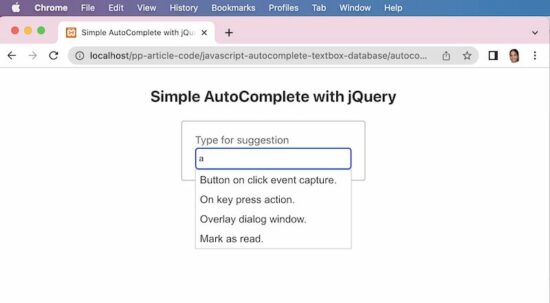
The below example has an idea for a quick script for enabling the autocomplete feature. It uses JavaScript jQuery and jQuery UI libraries to implement this easily.
The jQuery autocomplete() uses the PHP endpoint autocomplete.php script. Then, load the remote data into the textbox on the UI.
This PHP endpoint script reads the database results and forms the output JSON for the autocomplete textbox.
It receives the searched term from the UI and looks into the database for relevant suggestions.
autocomplete.php
<?php
$name = $_GET['term'];
$name = "%$name%";
$conn = mysqli_connect('localhost', 'root', '', 'phppot_autocomplete');
$sql = "SELECT * FROM tbl_post WHERE title LIKE ?";
$statement = $conn->prepare($sql);
$statement->bind_param('s', $name);
$statement->execute();
$result = $statement->get_result();
$autocompleteResult = array();
if (! empty($result)) { while ($row = $result->fetch_assoc()) { $autocompleteResult[] = $row["title"]; }
}
print json_encode($autocompleteResult);
?>
This database is for setting up the database created for this quick example. The next example also needs this database for displaying the autosuggest values.
Run the below database queries for getting a good experience with the above code execution.
CREATE TABLE `tbl_post` ( `id` int(11) UNSIGNED NOT NULL, `title` text DEFAULT NULL
) ENGINE=InnoDB DEFAULT CHARSET=utf8mb4; --
-- Dumping data for table `tbl_post`
-- INSERT INTO `tbl_post` (`id`, `title`) VALUES
(1, 'Button on click event capture.'),
(2, 'On key press action.'),
(3, 'Overlay dialog window.);
Example 2: Load autocomplete with ID
The AutoComplete function sends an additional parameter with the default term argument. That is to limit the number of results shown in the autocomplete textbox.
It returns the database results based on the searched term as a key-value pair. A JavaScript callback iterates the result and maps the key-value as label-value pair.
It is helpful when the result id is required while selecting a particular item from the autosuggest list.
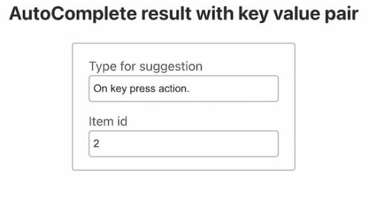
The below screenshot shows the item value and id is populated. This data is put into the textbox on selecting the autocomplete list item.
The below JavaScript code has two textboxes. One textbox is enabled with the autocomplete feature.
On typing into that textbox, the JavaScript autocomplete calls the server-side PHP script. The callback gets the JSON output returned by the PHP script.
This JSON data contains an association of dynamic results with their corresponding id. On selecting the autocomplete result item, the select callback function access the UI.item object.
Using this object, it gets the id and post title from the JSON data bundle. Then this JavaScript callback function targets the UI textboxes to populate the title and id of the selected item.
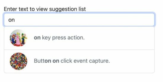
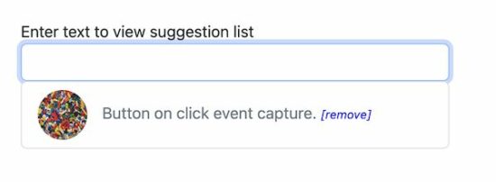
This example shows the autocomplete box with text and image data. The database for this example contains additional details like description and featured_image for the posts.
If you want a sleek and straightforward autocomplete solution with text, then use the above two examples.
This example uses BootStrap and plain JavaScript without jQuery. It displays recent searches on focusing the autocomplete textbox.
Create AutoComplete UI with Bootstrap and JavaScript Includes
See this HTML loads the autocomplete textbox and required JavaScript and CSS assets for the UI. The autocomplete.js handles the autosuggest request raised from the UI.
The autocomplete textbox has the onKeyPress and onFocus attributes. The onKeyPress attribute calls JavaScript to show an autosuggest list. The other attribute is for displaying recent searches on the focus event of the textbox.
Get the autosuggest list from the tbl_post database table
The below JavaScript function is called on the keypress event of the autocomplete field. In the previous examples, it receives a JSON response to load the dynamic suggestion.
In this script, it receives the HTML response from the endpoint. This HTML is with an unordered list of autosuggest items.
function showSuggestionList(searchInput) { if (searchInput.length > 1) { var xhttp = new XMLHttpRequest(); xhttp.open('POST', 'ajax-endpoint/get-auto-suggestion.php', true); xhttp.setRequestHeader("Content-type", "application/x-www-form-urlencoded"); xhttp.send("formData=" + searchInput); xhttp.onreadystatechange = function() { if (xhttp.readyState == 4 && xhttp.status == 200) { document.getElementById('auto-suggestion-box').innerHTML = xhttp.responseText; } } } else { document.getElementById('auto-suggestion-box').innerHTML = ''; }
}
ajax-endpoint/get-auto-suggestion.php
<?php
require_once __DIR__ . '/../lib/DataSource.php';
$dataSource = new DataSource(); if (isset($_POST["formData"])) { $searchInput = filter_var($_POST["formData"], FILTER_SANITIZE_STRING); $highlight = '<b>' . $searchInput . '</b>'; $query = "SELECT * FROM tbl_post WHERE title LIKE ? OR description LIKE ? ORDER BY id DESC LIMIT 15"; $result = $dataSource->select($query, 'ss', array( "%" . $searchInput . "%", "%" . $searchInput . "%" )); if (! empty($result)) { ?>
<ul class="list-group">
<?php foreach ($result as $row) { ?> <li class="list-group-item text-muted" data-post-id="<?php echo $row["id"]; ?>" onClick="addToHistory(this)" role="button"><img class="post-icon" src="<?php echo $row["featured_image"]; ?>" /><span> <?php echo str_ireplace($searchInput, $highlight, $row["title"]); ?> </span></li>
<?php } ?>
</ul>
<?php }
}
?>
Add to search history
When selecting the suggested list item, it triggers this JavaScript function on click.
This function reads the post id and title added to the HTML5 data attribute. Then passes these details to the server-side PHP script.
This PHP code removes the search instances stored in the tbl_search_history database. The delete request posts the record id to fire the delete action.
Solution: There are four simple ways to convert a list of dicts to a CSV file in Python.
Pandas: Import the pandas library, create a Pandas DataFrame, and write the DataFrame to a file using the DataFrame method DataFrame.to_csv('my_file.csv').
CSV: Import the csvmodule in Python, create a CSV DictWriter object, and write the list of dicts to the file in using the writerows() method on the writer object.
Python: Use a pure Python implementation that doesn’t require any library by using the Python file I/O functionality.
Reduce Problem: You can first convert the list of dicts to a list of lists and then use our related tutorial’s methods to write the list of lists to the CSV.
My preference is Method 1 (Pandas) because it’s simplest to use, concise, and most robust for different input types (numerical or textual).
Method 1: Pandas DataFrame to_csv()
You can convert a list of lists to a Pandas DataFrame that provides you with powerful capabilities such as the to_csv() method. This is the easiest method and it allows you to avoid importing yet another library (I use Pandas in many Python projects anyways).
You create a Pandas DataFrame—which is Python’s default representation of tabular data. Think of it as an Excel spreadsheet within your code (with rows and columns).
The DataFrame is a very powerful data structure that allows you to perform various methods. One of those is the to_csv() method that allows you to write its contents into a CSV file.
You set the index argument of the to_csv() method to False because Pandas, per default, adds integer row and column indices 0, 1, 2, …. Again, think of them as the row and column indices in your Excel spreadsheet. You don’t want them to appear in the CSV file so you set the arguments to False.
You set the and header argument to True because you want the dict keys to be used as headers of the CSV.
If you want to customize the CSV output, you’ve got a lot of special arguments to play with. Check out this article for a comprehensive list of all arguments.
You can convert a list of dicts to a CSV file in Python easily—by using the csv library. This is the most customizable of all four methods.
Here are the six easy steps to convert a list of dicts to a CSV with header row:
Import the CSV library with import csv.
Open the CSV file using the expression open('my_file.csv', 'w', newline=''). You need the newline argument because otherwise, you may see blank lines between the rows in Windows.
Create a csv.DictWriter() object passing the file and the fieldnames argument.
Set the fieldnames argument to the first dictionary’s keys using the expression salary[0].keys().
You can customize the CSV writer in its constructor (e.g., by modifying the delimiter from a comma ',' to a whitespace ' ' character). Have a look at the specification to learn about advanced modifications.
Method 3: Pure Python Without External Dependencies
If you don’t want to import any library and still convert a list of dicts into a CSV file, you can use standard Python implementation as well: it’s not complicated and very efficient.
This method is best if you won’t or cannot use external dependencies.
Open the file f in writing mode using the standard open() function.
Write the first dictionary’s keys in the file using the one-liner expression f.write(','.join(salary[0].keys())).
Iterate over the list of dicts and write the values in the CSV using the expression f.write(','.join(str(x) for x in row.values())).
Here’s the concrete code example:
salary = [{'Name':'Alice', 'Job':'Data Scientist', 'Salary':122000}, {'Name':'Bob', 'Job':'Engineer', 'Salary':77000}, {'Name':'Carl', 'Job':'Manager', 'Salary':119000}] # Method 3
with open('my_file.csv','w') as f: f.write(','.join(salary[0].keys())) f.write('\n') for row in salary: f.write(','.join(str(x) for x in row.values())) f.write('\n')
In the code, you first open the file object f. Then you iterate over each row and each element in the row and write the element to the file—one by one. After each element, you place the comma to generate the CSV file format. After each row, you place the newline character '\n'.
Note: to get rid of the trailing comma, you can check if the element x is the last element in the row within the loop body and skip writing the comma if it is.
A simple approach to convert a list of dicts to a CSV file is to first convert the list of dicts to a list of lists and then use the approaches discussed in the following article (code block given).
salary = [['Alice', 'Data Scientist', 122000], ['Bob', 'Engineer', 77000], ['Ann', 'Manager', 119000]] # Method 1
import csv
with open('file.csv', 'w', newline='') as f: writer = csv.writer(f) writer.writerows(salary) # Method 2
import pandas as pd
df = pd.DataFrame(salary)
df.to_csv('file2.csv', index=False, header=False) # Method 3
a = [[1, 2, 3], [4, 5, 6], [7, 8, 9]] import numpy as np
a = np.array(a)
np.savetxt('file3.csv', a, delimiter=',') # Method 4
with open('file4.csv','w') as f: for row in salary: for x in row: f.write(str(x) + ',') f.write('\n')
Coders get paid six figures and more because they can solve problems more effectively using machine intelligence and automation.
To become more successful in coding, solve more real problems for real people. That’s how you polish the skills you really need in practice. After all, what’s the use of learning theory that nobody ever needs?
You build high-value coding skills by working on practical coding projects!
Do you want to stop learning with toy projects and focus on practical code projects that earn you money and solve real problems for people?
If your answer is YES!, consider becoming a Python freelance developer! It’s the best way of approaching the task of improving your Python skills—even if you are a complete beginner.
If you just want to learn about the freelancing opportunity, feel free to watch my free webinar “How to Build Your High-Income Skill Python” and learn how I grew my coding business online and how you can, too—from the comfort of your own home.
Run the following command in your command line or PowerShell (Windows) or shell or terminal (macOS, Linux, Ubuntu) to install the csv-ical library:
pip install csv-ical
In some instances, you need to modify this command a bit to make it work. If you need more assistance installing the library, check out my detailed guide.
Create a new Python code file with the extension .py or a Jupyter Notebook with the file extension .ipynb. This creates a Python script or Jupyter Notebook that can run the code in Step 3 to conver the .ics.
Now, put the .ics file to be converted in the same folder as the newly-created Python script.
Use Jupyter Notebook to create a new .ipynb file
Step 3: Convert
This step consists of running the code doing these three things:
Create and initialize a Convert object
Read the .ics file
Create the CSV object and save it at the specified location
Here’s the full code:
from csv_ical import Convert # Create and initialize a Convert object
convert = Convert()
convert.CSV_FILE_LOCATION = 'my_file.csv'
convert.SAVE_LOCATION = 'my_file.ics' # Read the .ics file
convert.read_ical(convert.SAVE_LOCATION) # Create the CSV object and save it at the specified location
convert.make_csv()
convert.save_csv(convert.CSV_FILE_LOCATION)




 Learn More: If you want to learn about 7 Best Ways to Convert Dict to CSV in Python,
  Question: How to convert a


 If your answer is YES!, consider becoming a

 The key takeaway is that it is the settings of the weights and biases that establish how the network as a whole computes. In other words, the learning and memory of the network is encoded by the weights and biases.