Problem Formulation and Solution Overview

This article works with the fictitious Finxter database to retrieve three (3) specific users, via a SQLite query using the IN command.

To follow along, click here to download this file and move it into the current working directory.

---

Preparation

Add the following code to the top of the code snippet. This snippet will allow the code in this article to run error-free.

import sqlite3

Note: The SQLite library is built into Python and does not need to be installed but must be referenced.

---

Overview

The Finxter database file contains 25 records in tuple format. Below is a snippet from this file.

(30022145, 'Steve', 'Hamilton', 'Authority') (30022192, 'Amy', 'Pullister', 'Beginner') (30022331, 'Peter', 'Dunn', 'Basic Knowledge') (30022345, 'Marcus', 'Williams', 'Experienced Learner') (30022359, 'Alice', 'Miller', 'Authority') (30022361, 'Craig', 'Driver', 'Autodidact') ...

The structure of the users table is as follows:

DATA TYPE	FIELD NAME
INTEGER	FID
TEXT	First_Name
TEXT	Last_Name
TEXT	Rank

Now that the overview is complete, let’s connect to the database, filter, and output the results.

---

Connect to a SQLite Database

This code connects to an SQLite database and is placed inside a try/except statement to catch any possible errors.

try: conn = sqlite3.connect('finxter_users.db') cur = conn.cursor() except Exception as e: print(f'An error occurred: {e}.') exit()

The code inside the try statement executes first and attempts to connect to finxter_users.db. A Connection Object (conn), similar to below, is produced, if successful.

<sqlite3.Connection object at 0x00000194FFBC2140>

Next, the Connection Object created above (conn) is used in conjunction with the cursor() to create a Cursor Object. A Cursor Object (cur), similar to below, is produced, if successful.

<sqlite3.Cursor object at 0x0000022750E5CCC0>

Note: The Cursor Object allows interaction with database specifics, such as executing queries.

If the above line(s) fail, the code falls inside except capturing the error (e) and outputs this to the terminal. Code execution halts.

---

Prepare the SQLite Query

Before executing any query, you must decide the expected results and how to achieve this.

try: conn = sqlite3.connect('finxter_users.db') cur = conn.cursor() fid_list = [30022192, 30022450, 30022475] fid_tuple = tuple(fid_list) f_query = f'SELECT * FROM users WHERE FID IN {format(fid_tuple)}' except Exception as e: print(f'An error occurred: {e}.') exit()

In this example, the three (3) highlighted lines create, configure and save the following variables:

• fid_list: this contains a list of the selected Users’ FIDs to retrieve.
• fid_tuple: this converts fid_list into a tuple format. This is done to match the database format (see above).
• f_query: this constructs an SQLite query that returns all matching records when executed.

Query String Output

If f_query was output to the terminal (print(f_query)), the following would display. Perfect! That’s exactly what we want.

SELECT * FROM users WHERE FID IN (30022192, 30022450, 30022475)

---

Executing the SQLite Query

Let’s execute the query created above and save the results.

try: conn = sqlite3.connect('finxter_users.db') cur = conn.cursor() fid_list = [30022192, 30022450, 30022475] fid_tuple = tuple(fid_list) f_query = f'SELECT * FROM users WHERE FID IN {format(fid_tuple)}' results = cur.execute(f_query)

except Exception as e: print(f'An error occurred: {e}.') exit()

The highlighted line appends the execute() method to the Cursor Object and passes the f_query string as an argument.

If the execution was successful, an iterable Cursor Object is produced, similar to below.

<sqlite3.Cursor object at 0x00000224FF987A40>

---

Displaying the Query Results

The standard way to display the query results is by using a for a loop.
We could add this loop inside/outside the try/except statement.

try: conn = sqlite3.connect('finxter_users.db') cur = conn.cursor() fid_list = [30022192, 30022450, 30022475] fid_tuple = tuple(fid_list) f_query = f'SELECT * FROM users WHERE FID IN {format(fid_tuple)}' results = cur.execute(f_query)

except Exception as e: print(f'An error occurred: {e}.') exit() for r in results: print®

conn.close()

The highlighted lines instantiate a for loop to navigate the query results one record at a time and output them to the terminal.

Query Results

(30022192, 'Amy', 'Pullister', 'Beginner') (30022450, 'Leon', 'Garcia', 'Authority') (30022475, 'Isla', 'Jackson', 'Scholar')

Finally, the Connection Object created earlier needs to be closed.

---

Summary

In this article you learned how to:

• Create a Connection Object.
• Create a Cursor Object.
• Construct and Execute a SQLite Query.
• Output the results to the terminal.

We hope you enjoyed this article.

Happy Coding!

---

Programmer Humor

Programmer 1: We have a problem
Programmer 2: Let’s use RegEx!
Programmer 1: Now we have two problems

… yet – you can easily reduce the two problems to zero as you polish your “RegEx Superpower in Python“.

The name agg is short for aggregate. To aggregate is to summarize many observations into a single value that represents a certain aspect of the observed data.

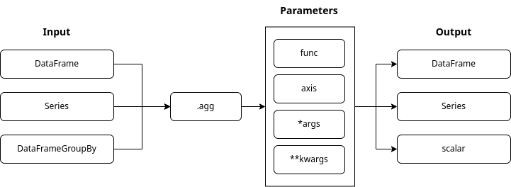
The .agg() function can process a dataframe, a series, or a grouped dataframe. It can execute many aggregation functions, e.g. ‘mean’, ‘max’,… in a single call along one of the axis. It can also execute lambda functions. Read on for examples.    

We will use a dataset of FIFA players. Find the dataset here.

Basic Setup using Jupyter Notebook

Let’s start by importing pandas and loading our dataset.

import pandas as pd

df_fifa_soccer_players = pd.read_csv('fifa_cleaned.csv')

df_fifa_soccer_players.head()

To increase readability, we will work with a subset of the data. Let’s create the subset by selecting the columns we want to have in our subset and create a new dataframe.

df_fifa_soccer_players_subset = df_fifa_soccer_players[['nationality', 'age', 'height_cm', 'weight_kgs', 'overall_rating', 'value_euro', 'wage_euro']]

df_fifa_soccer_players_subset.head()

Basic Aggregation

Pandas provides a variety of built-in aggregation functions. For example, pandas.DataFrame.describe. When applied to a dataset, it returns a summary of statistical values. 

df_fifa_soccer_players_subset.describe()

To understand aggregation and why it is helpful, let’s have a closer look at the data returned.

Example: Our dataset contains records for 17954 players. The youngest player is 17 years of age and the oldest player is 46 years old. The mean age is 25 years. We learn that the tallest player is 205 cm tall and the average player’s height is around 175 cm. With a single line of code, we can answer a variety of statistical questions about our data. The describe function identifies numeric columns and performs the statistical aggregation for us. Describe also excluded the column nationality that contains string values.

To aggregate is to summarize many observations into a single value that represents a certain aspect of the observed data.

Pandas provides us with a variety of pre-built aggregate functions.

Functions	Description
mean()	returns the mean of a set of values
sum()	returns the sum of a set of values
count()	returns the count of a set of values
std()	returns the standard deviation of a set of values
min()	returns the smallest value of a set of values
max()	returns the largest value of a set of values
describe()	returns a collection of statistical values of a set of values
size()	returns the size of a set of values
first()	returns the first value of a set of values
last()	returns the last value of a set of values
nth()	returns the nth value of a set of values
sem()	returns the standard error of the mean of a set of value
var()	returns the variance of a set of values
nunique()	returns the count of unique values of a set of values

Let’s use another function from the list above. We can be more specific and request the ‘sum’ for the ‘value_euro’ series. This column contains the market value of a player. We select the column or series ‘value_euro’ and execute the pre-build sum() function.

df_fifa_soccer_players_subset['value_euro'].sum()

# 43880780000.0

Pandas returned us the requested value. Let’s get to know an even more powerful pandas method for aggregating data.

The ‘pandas.DataFrame.agg’ Method

Function Syntax

The .agg() function can take in many input types. The output type is, to a large extent, determined by the input type. We can pass in many parameters to the .agg() function. 

The “func” parameter:

• is by default set to None 
• contains one or many functions that aggregate the data
• supports pre-defined pandas aggregate functions
• supports lambda expressions
• supports the dataframe.apply() method for specific function calls

The “axis” parameter:

• is by default set to 0 and applies functions to each column
• if set to 1 applies functions to rows
• can hold values:
  
  • 0 or ‘index’
  • 1 or ‘columns’

What about *args and **kwargs:

• we use these placeholders, if we do not know in advance how many arguments we will need to pass into the function
• when arguments are of the same type, we use *args
• When arguments are of different types, we use **kwargs.

Agg method on a Series

Let’s see the .agg() function in action. We request some of the pre-build aggregation functions for the ‘wage_euro’ series. We use the function parameter and provide the aggregate functions ‌we want to execute as a list. And let’s save the resulting series in a variable. 

wage_stats = df_fifa_soccer_players_subset['wage_euro'].agg(['sum', 'min', 'mean', 'std', 'max'])

print(wage_stats)

Pandas uses scientific notation for large and small floating-point numbers. To convert the output to a familiar format, we must move the floating point to the right as shown by the plus sign. The number behind the plus sign represents the amount of steps.

Let’s do this together for some values.

The sum of all wages is 175,347,000€ (1.753470e+08)

The mean of the wages is 9902.135€ (9.902135e+03)

We executed many functions on a series input source. Thus our variable ‘wage_stats’ is of the type Series because. 

type(wage_stats)

# pandas.core.series.Series

See below how to extract, for example, the ‘min’ value from the variable and the data type returned.

wage_stats_min = wage_stats['min']

print(wage_stats_min)

# 1000.0 print(type(wage_stats_min))

# numpy.float64

The data type is now a scalar.

If we execute a single function on the same data source (series), the type returned is a scalar.

wage_stats_max = df_fifa_soccer_players_subset['wage_euro'].agg('max')

print(wage_stats_max)

# 565000.0 print(type(wage_stats_max))

# numpy.float64

Let’s use one more example to understand the relation between the input type and the output type.

We will use the function “nunique” which will give us the count of unique nationalities. Let’s apply the function in two code examples. We will reference the series ‘nationality’ both times. The only difference will be the way we pass the function “nunique” into our agg() function.

nationality_unique_series = df_fifa_soccer_players_subset['nationality'].agg({'nationality':'nunique'})

print(nationality_unique_series)

# nationality 160

# Name: nationality, dtype: int64 print(type(nationality_unique_series))

# pandas.core.series.Series

When we use a dictionary to pass in the “nunique” function, the output type is a series.

nationality_unique_int = df_fifa_soccer_players_subset['nationality'].agg('nunique')

print(nationality_unique_int)

# 160 print(type(nationality_unique_int))

# int

When we pass the “nunique” function directly into agg() the output type is an integer.

Agg method on a DataFrame

Passing the aggregation functions as a Python list

One column represents a series. We will now select two columns as our input and so work with a dataframe.

Let’s select the columns ‘height_cm’ and ‘weight_kgs’.

We will execute the functions min(), mean() and max(). To select a two-dimensional data (dataframe), we need to use double brackets. We will round the results to two decimal points.

Let’s store the result in a variable.

height_weight = df_fifa_soccer_players_subset[['height_cm', 'weight_kgs']].agg(['min', 'mean', 'max']).round(2)

print(height_weight)

We get a data frame containing rows and columns. Let’s confirm this observation by checking the type of the ‘height_weight’ variable.

print(type(height_weight))

# pandas.core.frame.DataFrame

We will now use our newly created dataframe named ‘height_weight’ to use the ‘axis’ parameter. The entire dataframe contains numeric values.

We define the functions and pass in the axis parameter. I used the count() and sum() functions to show the effect of the axis parameter. The resulting values make little sense. This is also the reason why I do not rename the headings to restore the lost column names.

height_weight.agg(['count', 'sum'], axis=1)

We aggregated along the rows. Returning the count of items and the sum of item values in each row.

Passing the aggregation functions as a python dictionary

Now let’s apply different functions to the individual sets in our dataframe. We select the sets ‘overall_rating’ and ‘value_euro’. We will apply the functions std(), sem() and mean() to the ‘overall_rating’ series, and the functions min() and max() to the ‘value_euro’ series.

rating_value_euro_dict = df_fifa_soccer_players_subset[['overall_rating', 'value_euro']].agg({'overall_rating':['std', 'sem', 'mean'], 'value_euro':['min', 'max']})

print(rating_value_euro_dict)

The dataframe contains calculated and empty (NaN) values. Let’s quickly confirm the type of our output.

print(type(rating_value_euro_dict))

# pandas.core.frame.DataFrame

Passing the aggregation functions as a Python tuple

We will now repeat the previous example.

We will use tuples instead of a dictionary to pass in the aggregation functions. Tuple have limitations. We can only pass one aggregation function within a tuple. We also have to name each tuple. 

rating_value_euro_tuple = df_fifa_soccer_players_subset[['overall_rating', 'value_euro']].agg(overall_r_std=('overall_rating', 'std'),overall_r_sem=('overall_rating', 'sem'),overall_r_mean=('overall_rating', 'mean'),value_e_min=('value_euro', 'min'),value_e_max=('value_euro', 'max'))

print(rating_value_euro_tuple)

Agg method on a grouped DataFrame

Grouping by a single column

The ‘groupby’ method creates a grouped dataframe. We will now select the columns ‘age’ and ‘wage_euro’ and group our dataframe using the column ‘age’. On our grouped dataframe we will apply the agg() function using the functions count(), min(), max() and mean().

age_group_wage_euro = df_fifa_soccer_players_subset[['age', 'wage_euro']].groupby('age').aggage(['count', 'min', 'max', 'mean'])

print(age_group_wage_euro)

Every row represents an age group. The count value shows how many players fall into the age group. The min, max and mean values aggregate the data of the age-group members.

Multiindex

One additional aspect of a grouped dataframe is the resulting hierarchical index. We also call it multiindex.

We can see that the individual columns of our grouped dataframe are at different levels. Another way to view the hierarchy is to request the columns for the particular dataset.

print(age_group_wage_euro.columns)

Working with a multiindex is a topic for another blog post. To use the tools that we have discussed, let’s flatten the multiindex and reset the index. We need the following functions:

• droplevel()
• reset_index()

age_group_wage_euro_flat = age_group_wage_euro.droplevel(axis=1, level=0).reset_index()

print(age_group_wage_euro_flat.head())

The resulting dataframe columns are now flat. We lost some information during the flattening process. Let’s rename the columns and return some of the lost context.

age_group_wage_euro_flat.columns = ['age', 'athlete_count', 'min_wage_euro', 'max_wage_euro', 'mean_wage_euro']

print(age_group_wage_euro_flat.head())

Grouping by multiple columns

Grouping by multiple columns creates even more granular subsections.

Let’s use ‘age’ as the first grouping parameter and ‘nationality’ as the second. We will aggregate the resulting group data using the columns ‘overall_rating’ and ‘height_cm’. We are by now familiar with the aggregation functions used in this example.

df_fifa_soccer_players_subset.groupby(['age', 'nationality']).agg({'overall_rating':['count', 'min', 'max', 'mean'], 'height_cm':['min', 'max', 'mean']})

Every age group contains nationality groups. The aggregated athletes data is within the nationality groups.

Custom aggregation functions

We can write and execute custom aggregation functions to answer very specific questions.

Let’s have a look at the inline lambda functions.

Lambda functions are so-called anonymous functions. They are called this way because they do not have a name. Within a lambda function, we can execute multiple expressions. We will go through several examples to see lambda functions in action.

In pandas lambda functions live inside the “DataFrame.apply()” and the “Series.appy()” methods. We will use the DataFrame.appy() method to execute functions along both axes. Let’s have a look at the basics first.

Function Syntax

The DataFrame.apply() function will execute a function along defined axes of a DataFrame. The functions that we will execute in our examples will work with Series objects passed into our custom functions by the apply() method. Depending on the axes that we will select, the Series will comprise out of a row or a column or our data frame.

The “func” parameter:

• contains a function applied to a column or a row of the data frame

The “axis” parameter:

• is by default set to 0 and will pass a series of column data
• if set to 1 will pass a series of the row data
• can hold values:
  
  • 0 or ‘index’
  • 1 or ‘columns’

The “raw” parameter:

• is a boolean value
•  is by default set to False
• can hold values:
  
  • False -> a Series object is passed to the function
  • True -> a ndarray object is passed to the function

The “result_type” parameter:

• can only apply when the axis is 1 or ‘columns’
• can hold values:
  
  • ‘expand’
  • ‘reduce’
  • ‘broadcast’

 The “args()” parameter:

• additional parameters for the function as tuple

The **kwargs parameter:

• additional parameters for the function as key-value pairs

Filters

Let’s have a look at filters. They will be very handy as we explore our data.

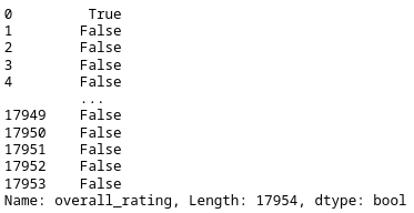
In this code example, we create a filter named filt_rating. We select our dataframe and the column overall_rating. The condition >= 90 returns True if the value in the overall_rating column is 90 or above.

Otherwise, the filter returns False.

filt_rating = df_fifa_soccer_players_subset['overall_rating'] >= 90

print(filt_rating)

The result is a Series object containing the index, and the correlated value of True or False.

Let’s apply the filter to our dataframe. We call the .loc method and pass in the filter’s name as a list item. The filter works like a mask. It covers all rows that have the value False. The remaining rows match our filter criteria of overall_rating >= 90.

df_fifa_soccer_players_subset.loc[filt_rating]

Lambda functions

Let’s recreate the same filter using a lambda function. We will call our filter filt_rating_lambda.

Let’s go over the code. We specify the name of our filter and call our dataframe. Pay attention to the double square brackets. We use them to pass a dataframe and not a Series object to the .appy() method.

Inside .apply() we use the keyword ‘lambda’ to show that we are about to define our anonymous function. The ‘x’ represents the Series passed into the lambda function.

The series contains the data from the overall_rating column. After the semicolumn, we use the placeholder x again. Now we apply a method called ge(). It represents the same condition we used in our first filter example “>=” (greater or equal).

We define the integer value 90 and close the brackets on our apply function. The result is a dataframe that contains an index and only one column of boolean values. To convert this dataframe to a Series we use the squeeze() method.

filt_rating_lambda = df_fifa_soccer_players_subset[['overall_rating']].apply(lambda x:x.ge(90)).squeeze()

print(filt_rating_lambda)

Let’s use our filter. Great, we get the same result as in our first filter example.

df_fifa_soccer_players_subset.loc[filt_rating_lambda]

We now want to know how many players our filter returned. Let’s first do it without a lambda function and then use a lambda function to see the same result. We are counting the lines or records.

df_fifa_soccer_players_subset.loc[filt_rating_lambda].count()

df_fifa_soccer_players_subset.apply(lambda x:x.loc[filt_rating_lambda]).count()

Great. Now let’s put us in a place where we actually need to use the apply() method and a lambda function. We want to use our filter on a grouped data-frame.

Let’s group by nationality to see the distribution of these amazing players. The output will contain all columns. This makes the code easier to read.

df_fifa_soccer_players_subset.groupby('nationality').loc[filt_rating_lambda]

Pandas tells us in this error message that we can not use the ‘loc’ method on a grouped dataframe object.

Let’s now see how we can solve this problem by using a lambda function. Instead of using the ‘loc’ function on the grouped dataframe we use the apply() function. Inside the apply() function we define our lambda function. Now we use the ‘loc’ method on the variable ‘x’ and pass our filter. 

df_fifa_soccer_players_subset.groupby('nationality').apply(lambda x:x.loc[filt_rating_lambda])

Axis parameter of the apply() function

Now let’s use the axis parameter to calculate the Body-Mass-Index (BMI) for these players. Until now we have used the lambda functions on the columns of our data.

The ‘x’ variable was a representation of the individual column. We set the axis parameter to ‘1’. The ‘x’ variable in our lambda function will now represent the individual rows of our data.

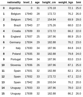
Before we calculate the BMI let’s create a new dataframe and define some columns. We will call our new dataframe ‘df_bmi’. 

df_bmi = df_fifa_soccer_players_subset.groupby('nationality')[['age', 'height_cm', 'weight_kgs']].apply(lambda x:x.loc[filt_rating_lambda])

print(df_bmi)

Now let’s reset the index.

df_bmi = df_bmi.reset_index()

print(df_bmi)

We calculate the BMI as follows. We divide the weight in kilogram by the square of the height in meters.

Let’s have a closer look at the lambda function. We define the ‘axis’ to be ‘1’. The ‘x’ variable now represents a row. We need to use specific values in each row. To define these values, we use the variable ‘x’ and specify a column name. At the beginning of our code example, we define a new column named ‘bmi’. And at the very end, we round the results.

df_bmi['bmi'] = df_bmi.apply(lambda x:x['weight_kgs']/((x['height_cm']/100)**2), axis=1).round()

print(df_bmi)

Great! Our custom function worked. The new BMI column contains calculated values.

Conclusion

Congratulations on finishing the tutorial. I wish you many great and small insights for your future data projects. I include the Jupyter-Notebook file, so you can experiment and tweak the code.

---

Nerd Humor