You may encounter a special ValueError when working with Python’s math module.
ValueError: math domain error
Python raises this error when you try to do something that is not mathematically possible or mathematically defined.
To understand this error, have a look at the definition of the domain:
“The domain of a function is the complete set of possible values of the independent variable. Roughly speaking, the domain is the set of all possible (input) x-values which result in a valid (output) y-value.” (source)
The domain of a function is the set of all possible input values. If Python throws the ValueError: math domain error, you’ve passed an undefined input into the math function. Fix the error by passing a valid input for which the function is able to calculate a numerical output.
Here are a few examples:
Python Math Domain Error Sqrt
The math domain error appears if you pass a negative argument into the math.sqrt() function. It’s mathematically impossible to calculate the square root of a negative number without using complex numbers. Python doesn’t get that and throws a ValueError: math domain error.
Here’s a minimal example:
from math import sqrt
print(sqrt(-1)) '''
Traceback (most recent call last): File "C:\Users\xcent\Desktop\Finxter\Blog\code.py", line 2, in <module> print(sqrt(-1))
ValueError: math domain error '''
You can fix the math domain error by using the cmath package that allows the creation of complex numbers:
from cmath import sqrt
print(sqrt(-1))
# 1j
Python Math Domain Error Log
The math domain error for the math.log() function appears if you pass a zero value into it—the logarithm is not defined for value 0.
Here’s the code on an input value outside the domain of the logarithm function:
from math import log
print(log(0))
The output is the math domain error:
Traceback (most recent call last): File "C:\Users\xcent\Desktop\Finxter\Blog\code.py", line 3, in <module> print(log(0))
ValueError: math domain error
You can fix this error by passing a valid input value into the math.log() function:
from math import log
print(log(0.000001))
# -13.815510557964274
This error can sometimes appear if you pass a very small number into it—Python’s float type cannot express all numbers. To pass a value “close to 0”, use the Decimal module with higher precision, or pass a very small input argument such as:
math.log(sys.float_info.min)
Python Math Domain Error Acos
The math domain error for the math.acos() function appears if you pass a value into it for which it is not defined—arccos is only defined for values between -1 and 1.
Here’s the wrong code:
import math
print(math.acos(2))
The output is the math domain error:
Traceback (most recent call last): File "C:\Users\xcent\Desktop\Finxter\Blog\code.py", line 3, in <module> print(math.acos(2))
ValueError: math domain error
You can fix this error by passing a valid input value between [-1,1] into the math.acos() function:
import math
print(math.acos(0.5))
# 1.0471975511965979
Python Math Domain Error Asin
The math domain error for the math.asin() function appears if you pass a value into it for which it is not defined—arcsin is only defined for values between -1 and 1.
Here’s the erroneous code:
import math
print(math.asin(2))
The output is the math domain error:
Traceback (most recent call last): File "C:\Users\xcent\Desktop\Finxter\Blog\code.py", line 3, in <module> print(math.asin(2))
ValueError: math domain error
You can fix this error by passing a valid input value between [-1,1] into the math.asin() function:
import math
print(math.asin(0.5))
# 0.5235987755982989
Python Math Domain Error Pow
The math domain error for the math.pow(a,b) function to calculate a**b appears if you pass a negative base value into it and try to calculate a negative power of it. The reason it is not defined is that any negative number to the power of 0.5 would be the square number—and thus, a complex number. But complex numbers are not defined by default in Python!
import math
print(math.pow(-2, 0.5))
The output is the math domain error:
Traceback (most recent call last): File "C:\Users\xcent\Desktop\Finxter\Blog\code.py", line 3, in <module> print(math.pow(-2, 0.5))
ValueError: math domain error
If you need a complex number, ab must be rewritten into eb ln a. For example:
import numpy as np
import matplotlib.pyplot as plt # Plotting y = log(x)
fig, ax = plt.subplots()
ax.set(xlim=(-5, 20), ylim=(-4, 4), title='log(x)', ylabel='y', xlabel='x')
x = np.linspace(-10, 20, num=1000)
y = np.log(x) plt.plot(x, y)
This is the graph of log(x). Don’t worry if you don’t understand the code, what’s more important is the following point. You can see that log(x) tends to negative infinity as x tends to 0. Thus, it is mathematically meaningless to calculate the log of a negative number. If you try to do so, Python raises a math domain error.
>>> math.log(-10)
Traceback (most recent call last): File "<stdin>", line 1, in <module>
ValueError: math domain error
Where to Go From Here?
Enough theory, let’s get some practice!
To become successful in coding, you need to get out there and solve real problems for real people. That’s how you can become a six-figure earner easily. And that’s how you polish the skills you really need in practice. After all, what’s the use of learning theory that nobody ever needs?
Practice projects is how you sharpen your saw in coding!
Do you want to become a code master by focusing on practical code projects that actually earn you money and solve problems for people?
Then become a Python freelance developer! It’s the best way of approaching the task of improving your Python skills—even if you are a complete beginner.
This chapter from my upcoming book “From One to Zero” (to appear with NoStarch 2021) teaches you a well-known but still undervalued idea. The idea is to build a minimum viable product (in short: MVP) to test and validate your hypotheses quickly without losing a lot of time in implementation. In particular, you’ll learn how to apply the idea of radically reducing complexity in the software development cycle when creating value through software.
Stealth Mode of Programming
If you’re like me, you know what may be called the “stealth mode” of programming (see Figure 4-1). Many programmers fall victim to it, and it goes as follows: you come up with a wonderful idea of a computer program that will change the world—with the potential to become the next Google. Say you discovered that more and more people start coding, and you want to serve those by creating a machine-learning-enhanced search engine for code discovery. Sounds great? You think so—and you start coding enthusiastically on your idea a few nights in a row.
Figure 4-1: The stealth mode of programming.
But does this strategy work? Here’s a likely outcome of following the stealth mode of programming:
You quickly develop the prototype, but it doesn’t look right. So, you dive into design and optimize the design. Then, you try the search engine, and the recommendation results are not relevant for many search terms. For example, when searching for “Quicksort”, you obtain a “MergeSort” code snippet with a comment "# This quickly sorts the list". So, you keep tweaking the models. But each time you improve the results for one keyword, you create new problems for other search results. You’re never quite happy with the result, and you don’t feel like you can present your crappy code search engine to the world for three reasons. First, nobody will find it useful. Second, the first users will create negative publicity around your website because it doesn’t feel professional and polished. And third, if competitors see your poorly implemented concept, they’ll steal it and implement it in a better way. These depressing thoughts cause you to lose faith and motivation, and your progress on the app drops significantly.
Let’s analyze what can and will go wrong in the stealth mode of programming shown in Figure 4-2.
Figure 4-2: Common pitfalls in the stealth mode of programming
Pitfalls
There are many common pitfalls in the stealth mode of programming. Here are four of the more common ones:
Losing Motivation: As long as you’re in stealth mode, nobody can see you. Nobody knows about the great tool you’re implementing. You’re alone with your idea, and doubts will pop up regularly. Maybe you’re strong enough to resist the doubts initially—while your initial enthusiasm for the project is big enough. But the longer you’ll work on your project the more doubts will come into your mind. Your subconsciousness is lazy and seeks reasons not to do the work. You may find a similar tool. Or you may even doubt that your tool will be useful in the first place. You may start to believe that it cannot be done. If only one early adopter of your tool would have provided you some encouraging words, you’d probably stayed motivated. But, as you’re in stealth mode, nobody is going to encourage you to keep working. And, yes, nobody is paying you for your work. You have to steal time from your friends, your kids, your wife. Only a minority of people will sustain such a psychological drain. Most will simply lose motivation—the longer the stealth mode, the smaller the motivation to work on the project.
Getting Distracted: Even if you manage to stay motivated to work on the project for an extended period without any real-world feedback—there’s another powerful enemy: your daily distractions. You don’t live in a vacuum. You work in your day job, you spend time with family and friends, and other ideas will pop into your mind. Today, your attention is a rare good sought by many devices and services. While you work on one project, you’ll have ideas for other projects, and the grass-is-greener effect will kick in: many other projects seem to be so much more attractive! It takes a very disciplined person to manage these distractions, protect their working time, and stay focused on one project until they reach completion.
Taking Longer: Another powerful enemy is wrong planning. Say you initially plan that the project takes one month if you work on it for two hours every day. That’s 60 hours of estimated working time. Lost motivation and distractions will probably cause you to average only one hour every day, so it already doubles the project’s duration. However, other factors are responsible for underestimating the project duration: unexpected events and bugs take much more time than anticipated. You must learn new things to finish the project—and learning takes time. Especially when you mix learning time with answering Smartphone messages and notifications, emails, and phone calls. It’s tough to estimate how much learning time you need correctly. And even if you already know everything you need to know to finish the project, you likely run into unforeseen problems or bugs in your code. Or other features may pop into your mind that demand to be implemented. An infinite number of factors will increase your anticipated project duration—and hardly any will reduce it. But it is getting worse: if your project takes longer than anticipated, you’ll lose even more motivation, and you’ll face even more distractions causing a negative spiral towards project failure.
Delivering Too Little Value: Say you manage to overcome the phases of low motivation. You learn what you need, stay focused, and avoid any distraction for as long as it takes to finish the code. You finally launch your project, and—nothing happens. Only a handful of users even check out your project, and they’re not enthusiastic about it. The most likely outcome of any software project is silence—an absence of positive or negative feedback. You’ll wonder why nobody writing in with some constructive or even destructive feedback. Nobody seems to care. There are many reasons for this. A common reason is that your product doesn’t deliver the specific value the users demand. It’s almost impossible to find the so-called product-market-fit in the first shot. Well, even if you’d have found product-market-fit and users would generally value your software, you don’t yet have a marketing machine to sell it. If 5% of your visitors would buy the product, you could consider it a huge success. However, a 5% conversion rate means that 19 out of 20 people won’t buy the product! Did you expect a million-dollar launch? Hardly so; your software sells to one person in the first 20 days leading to an ultimate income of $97. And you’ve spent hundreds of hours implementing it. Discouraged by the results, you quickly give up the idea of creating your own software and keep working for your boss.
The likelihood of failure is high in the stealth mode of programming. There’s a negative feedback loop in place: if you stumble because of any of the discussed reasons, the code project will take you longer to finish—and you’ll lose even more motivation, which increases your chances of stumbling. Don’t underestimate the power of this negative feedback loop. Every programmer knows it very well, and it is why so many code projects never see the light of the day. So much time, effort, value is lost because of it. Individual and even teams of programmers may spend years of their lives working in the stealth mode of programming—only to fail early or find out that nobody wants their software product.
Reality Distortion
You would think that if programmers spend so much time working on a software project, they’d at least know that their users will find the end product valuable. But this is not the case. When they are sunk in the stealth mode of programming, programmers don’t get any feedback from the real world—a dangerous situation. They start to drift away from reality, working on features nobody asked for, or nobody will use.
You may ask: how can that happen? The reason is simple: your assumptions make it so. If you work on any project, you have a bunch of assumptions such as who the users will be, what they do for a living, what problems they face, or how often they will use your product. Years ago, when I was creating my Finxter.com app to help users learn Python by solving rated code puzzles, I assumed that most users are computer science students because I was one (reality: most users are not computer scientists). I assumed that people would come when I released the app (reality: nobody came initially). I assumed that people would share their successes on Finxter via their social media accounts (reality: only a tiny minority of people shared their coding ranks). I assumed that people would submit their own code puzzles (reality: from hundreds of thousands of users, only a handful submitted code puzzles). I assumed that people wanted a fancy design with colors and images (reality: a simple geeky design lead to improved usage behavior). All those assumptions lead to concrete implementation decisions. Implementing each feature—even the ones nobody wanted—had cost me tens, sometimes hundreds of hours. If I knew better, I could have tested these assumptions before spending lots of time working on them. I could have asked for feedback and prioritized implementing the features valued by the highly engaged users. Instead, I spent one year in stealth mode to develop a prototype with way too many features to test some of those hypotheses or assumptions.
Complexity — A Productivity Killer
There’s another problem with the stealth mode of programming: unnecessary complexity. Say you implement a software product consisting of four features (see Figure 4-3). You’ve been lucky—the market accepted it. You’ve spent considerable time implementing those four features, and you take the positive feedback as a reinforcement for all four features. All future releases of the software product will contain those four features—in addition to the future features you’ll add to the software product.
Figure 4-3: A valuable software product consisting of four features
However, by releasing the package of four features at once, you don’t know whether the market would’ve accepted any subset of features (see Figure 4-4).
Figure 4-4: Which subsets of features would have been accepted by the market?
Feature 1 may be completely irrelevant—even though it took you the most time to implement. At the same time, Feature 4 may be a highly valuable feature that the market demands. There are 2n different combinations of software product packages out of n features. How can you possibly know which is value and which is waste if you release them as feature bundles?
The costs of implementing the wrong features are already high. However, releasing feature bundles leads to cumulative costs of maintaining unnecessary features for all future versions of the product. Why? There are many reasons:
Every line of code slows down your understanding of the complete project. You need more time to “load” the whole project in your mind, the more features you implement.
Each feature may introduce a new bug in your project. Think of it this way: a given feature will crash your whole code base with a certain likelihood.
Each line of code causes the project to open, load, and compile more slowly. It’s a small but certain cost that comes with each new line of code.
When implementing Feature n, you must go over all previous Features 1, 2, …, n-1 and ensure that Feature n doesn’t interfere with their functionality.
Every new feature results in new (unit) tests that must compile and run before you can release the next version of the code.
Every added feature makes it more complicated for a new coder to understand the codebase, which increases learning time for new coders that join the growing project.
This is not an exhaustive list, but you get the point. If each feature increases your future implementation costs by X percent, maintaining unnecessary features can result in orders of magnitude difference in coding productivity. You cannot afford to systematically keep unnecessary features in your code projects!
So, you may ask: How do you overcome all these problems? If the stealth mode of programming is unlikely to succeed—then what is?
Minimum Viable Product — Release Early and Often
The solution is simple—quite literally. Think about how you can simplify the software, how you can get rid of all features but one, and how you can build a minimum viable product that accomplishes the same validation of your hypotheses as the “full” implementation of your ideas would have accomplished. Only if you know what features the marketplace accepts—and which hypotheses are true—should you add more features and more complexity. But at all costs, avoid complexity. Formulate an explicit hypothesis—such as users enjoy solving Python puzzles—and create a product that validates only this hypothesis. Remove all features that don’t help you validate this hypothesis. After all, if users don’t enjoy solving Python puzzles, why even proceed with implementing the Finxter.com website? What would have been the minimum viable product for Finxter? Well, I’ve thought about this, and I’d say it would have been a simple Instagram account that shares code puzzles and checks if the Python community enjoys solving them. Instead of spending one year writing the Finxter app without validation, I should’ve spent a few weeks or even months sharing puzzles on a social network. Then, I should’ve taken the learnings from interacting with the community and build a second MVP (the first one being the social media account) with slightly more functionality. Gradually, I’d built the Finxter app in a fraction of the time and with a fraction of the unnecessary features I’ve implemented and removed again in a painful process of figuring out which features are valuable and which are waste. The lesson of building a minimum viable product stripped from all unnecessary features is one I’ve learned the hard way.
Figure 4-5 sketches this gold standard of software development and product creation. First, you find product-market-fit through iteratively launching minimum viable products until users love it. The chained launches of MVPs build interest over time and allow you to incorporate user feedback to gradually improve the core idea of your software. As soon as you’ve reached product-market fit, you add new features—one at a time. Only if a feature can prove that it improves key user metrics, it remains in the product.
Figure 4-5: Two phases of software development: (1) Find product-market-fit through iterative MVP creation & build interest over time. (2) Scale-up by adding and validating new features through carefully designed split tests.
The term minimum viable product (MVP) was coined by Frank Robinson in 2001. Eric Ries popularized the term in his best-selling book Lean Startup. Since then, the concept has been tested by thousands of very successful companies in the software industry (and beyond). A famous example is the billion-dollar company Dropbox. Instead of spending lots of time and effort on an untested idea to implement the complicated Dropbox functionality of synchronizing folder structures into the cloud—that requires a tight integration in different operating systems and a thorough implementation of burdersome distributed systems concepts such as replica synchronization—the founders validated the idea with a simple product video even though the product they made a video about didn’t even exist at the time. Countless iterations followed on top of the validated Dropbox MVP to add more helpful features to the core project that simplify the lives of their users.
MVP Concept
Let’s have a more in-depth look at the MVP concept next, shall we?
A minimum viable product in the software sense is code that is stripped from all features to focus on the core functionality. For Finxter, it would have been a social media account centered around code puzzles. After that validation was successful, the next MVP would have been a simple app that does nothing but present code puzzles. You’d successively add new features such as videos and puzzle selection techniques extending the MVP functionality based on user need and early adopters’ feedback. For Dropbox, the first MVP was the video—and after successful validation, the second MVP was created building on the customer insight from the first MVP (e.g., a cloud storage folder for Windows but no more). For our code search engine example, the MVP could be a video shared via paid advertisement channels. I know you want to start coding right away on the search engine—but don’t do it until you have a clear concept that differentiates itself from other code search engines and you have a clear plan on how to focus. By working on your MVP concept before you dive into the code, you’ll not only save lots of time, but you stay nimble enough to find product-market-fit. Even the minimal form of your software will already satisfy your market’s needs and desires if you find product-market-fit. The market signals that they love and value your product, and people tell each other about your software product. Yes, you can achieve product-market-fit with a simple, well-crafted MVP—and by iteratively building and refining your MVPs. The term to describe this strategy of searching for the right product via a series of MVPs is called rapid prototyping. Instead of spending one year to prepare your big one-time launch, you launch 12 prototypes in 12 months. Each prototype builds on the learnings from the previous launches, and each is designed to bring you maximal learning in minimal time and with minimum effort. You release early and often!
Product-Market-Fit
One idea of building your MVPs to find product-market-fit is based on the theory that your product’s early adopters are more forgiving than the general market. Those people love new and unfinished products because it makes them feel special—they’re part of a new and emerging technology. They value products more based on their potential than the actual implementation. After all, they identify with being early adopters, so they must accept half-baked products. This is what you’re providing them with: rough, sketchy products with a great story on what this product could be. You reduce functionality, sometimes even fake the existence of a specific feature. Jeff Bezos, the founder of Amazon, initially faked to have individual books in stock to satisfy his customers and start the learning loop. When people ordered these books, he bought them manually from his local book publisher and forwarded them to his customers. True MVP-thinking!
Pillars MVP
If you’re building your first software based on MVP thinking, consider these four pillars: functionality, design, reliability, and usability.[1]
Functionality: The product provides a clearly-formulated function to the user, and it does it well. The function doesn’t have to be provided with great economic efficiency. If you sold a chat bot that was really you chatting with the user yourself, you’d still provide the functionality of high-quality chatting to the user—even though you haven’t figured out how to provide this functionality in an economically feasible way.
Design: The product is well-designed and focused, and it supports the value proposition of the product. This is one of the common mistakes in MVP generation—you create a poorly-designed MVP website and wonder why you never achieve product-market-fit. The design can be straightforward, but it must support the value proposition. Think Google search—they certainly didn’t spend lots of effort on design when releasing their first version of the search engine. Yet, the design was well-suited for the product they offered: distraction-free search.
Reliability: Only because the product is supposed to be minimal; this doesn’t mean it can be unreliable. Make sure to write test cases and test all functions in your code rigorously. Otherwise, your learnings from the MVP will be diluted by the negative user experience that comes from bad reliability. Remember: you want to maximize learning with minimal effort. But if your software product is full of bugs—how can you learn anything from the user feedback? The negative emotions could’ve all come from the error messages popping up in their web browsers.
Usability: The MVP is easy to use. The functionality is clearly articulated, and the design supports it. Users don’t need a lot of time figuring out what to do or on which buttons to click. The MVP is responsive and fast enough to allow fluent interactions. It is usually simpler to achieve superb usability with a focused, minimalistic product because a page with one button and one input field is easy to use. Again, the Google search engine’s initial prototype is so usable that it lasted for more than two decades.
A great MVP is well-designed, has great functionality (from the user’s perspective), is reliable and well-tested, and provides good usability. It’s not a crappy product that doesn’t communicate and provide unique value. Many people frequently misunderstand this characteristic of MVPs: they wrongly assume that an MVP provides little value, bad usability, or a lazy design. However, the minimalist knows that the reduced effort comes from a rigorous focus on one core functionality rather than from lazy product creation. For Dropbox, it was easier to create a stunning video than to implement the stunning service. The MVP was a high-quality product with great functionality, design, reliability, and usability nonetheless. It was only easier to accomplish these pillars in a video than in a software product!
Advantages
Advantages of MVP-driven software design are manifold. You can test your hypotheses as cheaply as possible. Sometimes, you can avoid writing code for a long time—and even if you do have to write code, you minimize the amount of work before gathering real-world feedback. This not only gives you clues on which features provide the best value for your users, but it also reduces waste and provides you with fast learning and a clear strategy for continuous improvement. You need much less time writing code and finding bugs—and if you do, you’ll know that this activity is highly valuable for your users. Any new feature you ship to users provides instant feedback, and the continuous progress keeps you and your team motivated to crank out feature after feature. This dramatically minimizes the risks you’re exposed to in the stealth mode of programming. Furthermore, you reduce the maintenance costs in the future because it reduces the complexity of your code base by a long shot—and all future features will be easier and less error prone. You’ll make faster progress, and implementation will be easier throughout the life of your software—which keeps you in a motivated state and on the road to success. Last but not least, you’ll ship products faster, earn money from your software faster, and build your brand in a more predictable, more reliable manner.
Split Testing
The final step of the software creation process is split testing: you not simply launch a product to the user base and hope that it delivers the value. Instead, you launch the new product with the new feature to a fraction of your users (e.g., 50%) and observe the implicit and explicit response. Only if you like what you see—for example, the average time spent on your website increases—you keep the feature. Otherwise, you reject it and stay with the simpler product without the feature. This is a sacrifice because you spend much time and energy developing the feature. However, it’s for the greater good because your product will remain as simple as possible, and you remain agile, flexible, and efficient when developing new features in the future—without the baggage of older features that nobody needs. By using split tests, you engage in data-driven software development. If your test is successful, you’ll ship more value to more people. You add one feature at a time if adding this feature leads to your vision—You’re on a path to progress with incremental improvements by doing less.
Low-Hanging Fruits & Rapid Greedy Progress
Figure 4-6: Two different ways of creating a software project by implementing a set of features: (Good) High-value low-effort features first; (Bad) Low-value, high-effort features first
Figure 4-6 shows two different ways of approaching a software project. Given is a fixed set of features—the horizontal length of a feature defines the time duration of implementing the feature, and the vertical length defines the value the feature delivers to the user. You can now either prioritize the high-value, low-effort features or prioritize the low-value, high-effort features. The former leads to rapid progress at the beginning of the project phase. The latter leads to rapid progress towards the end of the project phase. Theoretically, both lead to the same resulting software product delivering the same value to users. However, life is what happens if you plan—it’ll play out differently: the team that prioritizes the low-value, high-effort features won’t get any encouragement or feedback from the real world for an extended period. Motivation drops, progress comes to a halt, the project will likely die. The team that prioritizes high-value, low-effort features develops a significant momentum towards more value, gets user feedback quickly, and is far more likely to push the project to completion. They may also decide to skip the low-value, high-effort features altogether, replacing them with new high-value features obtained from the feedback of early adopters. It is surprising how far you can go by reaping only the low-hanging fruits!
Is Your Idea Special? You May Not Like The Truth
A common counterarguments against rapid prototyping and for the stealth mode of programming is that people assume their idea is so special and unique that if they release it in the raw form, as a minimum viable product, it will get stolen by larger and more powerful companies—that implement it in a better way. Frankly, this is such a poor way of thinking. Ideas are cheap; execution is king. Any given idea is unlikely to be unique. There are billions of people with trillions of ideas in their collective minds. And you can be quite sure that your idea has already been thought of by some other person. The ideas are out there, and nobody can stop their spread. Instead of reducing competition, the fact that you engage in the stealth mode of programming may even encourage others to work on the idea as well—because they assume like you that nobody else has already thought of it. For an idea to succeed, it takes a person to push it into reality. If you fast forward a few years, the person that will have succeeded will be the one who took quick and decisive action, who released early and often, incorporated feedback from real users and gradually improved their software by building on the momentum of previous releases. Keeping the idea “secret”—even if you could accomplish this in the first place—would simply restrict its growth potential and reduces its chances for success because it cannot be polished by dynamic execution and real-world feedback.
Summary
Envision your end product and think about the need of your users before you write any line of code. Work on your MVP and make it valuable, well-designed, responsive, and usable. Remove all features but the ones that are absolutely necessary to maximize your learnings. Focus on one thing at a time. Then, release an MVP quickly and often—improve it over time by gradually testing and adding more features. Less is more! Spend more time thinking about the next feature to implement than actually implementing each feature. Every feature incurs not only direct but also indirect implementation costs for all features to come in the future. Use split testing to test the response to two product variants at a time and quickly discard features that don’t lead to an improvement in your key user metrics such as retention, time on page, or activity. This leads to a more holistic approach to business—acknowledging that software development is only one step in the whole product creation and value delivery process.
In the next chapter, you’ll learn why and how to write clean and simple code—but remember: not writing unnecessary code is the surest way to clean and simple code!
Do you want to develop the skills of a well-rounded Python professional—while getting paid in the process? Become a Python freelancer and order your book Leaving the Rat Race with Python on Amazon (Kindle/Print)!
Return the shape of an array or array_like object a.
Argument
Data Type
Description
a
array_like
NumPy array or Python list for which the shape should be returned. If it is a NumPy array, it returns the attribute a.shape. If it is a Python list, it returns a tuple of integer values defining the number of elements in each dimension if you would’ve created a NumPy array from it.
Return Value: shape — a tuple of integers that are set to the lengths of the corresponding array dimensions.
Examples
The straightforward example is when applied to a NumPy array:
>>> import numpy as np
>>> a = np.array([[1, 2], [3, 4]])
>>> np.shape(a)
(2, 2)
You import the NumPy library and create a two-dimensional array from a list of lists. If you pass the NumPy array into the shape function, it returns a tuple with two values (=dimensions). Each dimension stores the number of elements in this dimension (=axis). As it is a 2×2 quadratic matrix, the result is (2,2).
The following shape is another example of a multi-dimensional array:
The shape is now (2, 4) with two rows and four columns.
np.shape() vs array.shape
Note that the result of np.shape(b) and b.shape is the same if b is a NumPy array. If b isn’t a NumPy array but a list, you cannot use b.shape as lists don’t have the shape attribute. Let’s have a look at this example:
The np.shape() function returns the same shape tuple—even if you pass a nested list into the function instead of a NumPy array.
But if you try to access the list.shape attribute, NumPy throws the following error:
>>> b.shape
Traceback (most recent call last): File "<pyshell#9>", line 1, in <module> b.shape
AttributeError: 'list' object has no attribute 'shape'
So, the difference between np.shape() and array.shape is that the former can be used for all kinds of array_like objects while the latter can only be used for NumPy arrays with the shape attribute.
Do you want to become a NumPy master? Check out our interactive puzzle book Coffee Break NumPy and boost your data science skills! (Amazon link opens in new tab.)
The .polyfit() function, accepts three different input values: x, y and the polynomial degree. Arguments x and y correspond to the values of the data points that we want to fit, on the x and y axes, respectively. The third parameter specifies the degree of our polynomial function. For example, to obtain a linear fit, use degree 1.
What is Curve Fitting?
Curve fitting consists in building a mathematical function that is able to fit some specific data points. Most of the times, the fitting equation is subjected to constraints; moreover, it is also possible to make initial guess for providing useful starting points for the estimation of the fitting parameters, this latter procedure has the advantage of lowering the computational work. In this article we will explore the NumPy function .polyfit(), which enables to create polynomial fit functions in a very simple and immediate way.
Linear fit
The simplest type of fit is the linear fit (a first-degree polynomial function), in which the data points are fitted using a straight line. The general equation of a straight line is:
y = mx + q
Where “m” is called angular coefficient and “q” intercept. When we apply a linear fit, we are basically searching the values for the parameters “m” and “q” that yield the best fit for our data points. In Numpy, the function np.polyfit() is a very intuitive and powerful tool for fitting datapoints; let’s see how to fit a random series of data points with a straight line.
In the following example, we want to apply a linear fit to some data points, described by the arrays x and y. The .polyfit() function, accepts three different input values: x, y and the polynomial degree. While x and y correspond to the values of the data points that we want to fit, on the x and y axes, respectively; the third parameter specifies the degree of our polynomial function. Since we want a linear fit, we will specify a degree equal to 1. The outputs of the polyfit() function will be a list containing the fitting parameters; the first is the one that in the function is multiplied by the highest degree term; the others then follow this order.
import numpy as np
from numpy import random #it will be useful for generating some random noise (on purpose) in the data points that we want to fit
import matplotlib.pyplot as plt #for plotting the data #---LINEAR FIT---- #generate the x array
x = np.linspace(0,60,60) # generate an array of 60 equally space points #generate the y array exploiting the random.randint() function to introduce some random noise
y = np.array([random.randint(i-2, i+2) for i in x]) #each element is a random number with value between +-2 the respective x axis value #Applying a linear fit with .polyfit()
fit = np.polyfit(x,y,1)
ang_coeff = fit[0]
intercept = fit[1]
fit_eq = ang_coeff*x + intercept #obtaining the y axis values for the fitting function #Plotting the data
fig = plt.figure()
ax = fig.subplots()
ax.plot(x, fit_eq,color = 'r', alpha = 0.5, label = 'Linear fit')
ax.scatter(x,y,s = 5, color = 'b', label = 'Data points') #Original data points
ax.set_title('Linear fit example')
ax.legend()
plt.show()
As mentioned before, the variable fit will contain the fitting parameters. The first one is the angular coefficient, the last one the intercept. At this point, in order to plot our fit, we have to build the y-axis values from the obtained parameters, using the original x-axis values. In the example, this step is described by the definition of the fit_eqvariable. The last remaining thing is to plot the data and the fitting equation. The result is:
Polynomial fit of second degree
In this second example, we will create a second-degree polynomial fit. The polynomial functions of this type describe a parabolic curve in the xy plane; their general equation is:
y = ax2+ bx + c
where a, b and c are the equation parameters that we estimate when generating a fitting function. The data points that we will fit in this example, represent the trajectory of an object that has been thrown from an unknown height. Exploiting the .polyfit() function, we will fit the trajectory of the falling object and we will also obtain an estimate for its initial speed in the x-direction, v0.
#-----POLYNOMIAL FIT----
x = np.array([1.2,2.5,3.4,4.0,5.4,6.1,7.2,8.1,9.0,10.1,11.2,12.3,13.4,14.1,15.0]) # x coordinates
y = np.array([24.8,24.5,24.0,23.3,22.4,21.3,20.0,18.5,16.8,14.9,12.8,10.5,8.0,5.3,2.4]) # y coordinates
fit = np.polyfit(x, y, 2)
a = fit[0]
b = fit[1]
c = fit[2]
fit_equation = a * np.square(x) + b * x + c
#Plotting
fig1 = plt.figure()
ax1 = fig1.subplots()
ax1.plot(x, fit_equation,color = 'r',alpha = 0.5, label = 'Polynomial fit')
ax1.scatter(x, y, s = 5, color = 'b', label = 'Data points')
ax1.set_title('Polynomial fit example')
ax1.legend()
plt.show()
Once initialized the x and y arrays defining the object trajectory, we apply the function .polyfit(), this time inserting “2” as degree of the polynomial fit function. This is because the trajectory of a falling object can be described by a second-degree polynomial; in our case the relation between the x and y coordinates is given by:
y = y0 – ½ (g/ v02)x2
where y0 is the initial position (the height from which the object has been thrown), g the acceleration of gravity ( ̴9.81 m/s2) and v0 the initial speed (m/s) in the x-direction (visit: https://en.wikipedia.org/wiki/Equations_for_a_falling_body for more details). We then assign at the variables a, b and cthe value of the 3 fitting parameters and we define fit_equation, the polynomial equation that will be plotted; the result is:
If we now print the three fitting parameters, a,b and c, we obtain the following values: a = -0.100 , b = 0.038, c = 24.92. In the equation describing the trajectory of a falling body there is no b term; since the fit is always an approximation of the real result, we will always get a value for all the parameters; however we shall notice that the value of our b term is much smaller than the others and can be somehow neglected, when comparing our fit with the equation describing the physics of the problem. The c term represents the initial height (y0) while the a term describes the quantity – ½ (g/ v02). Hence, the initial velocity v0is given by:
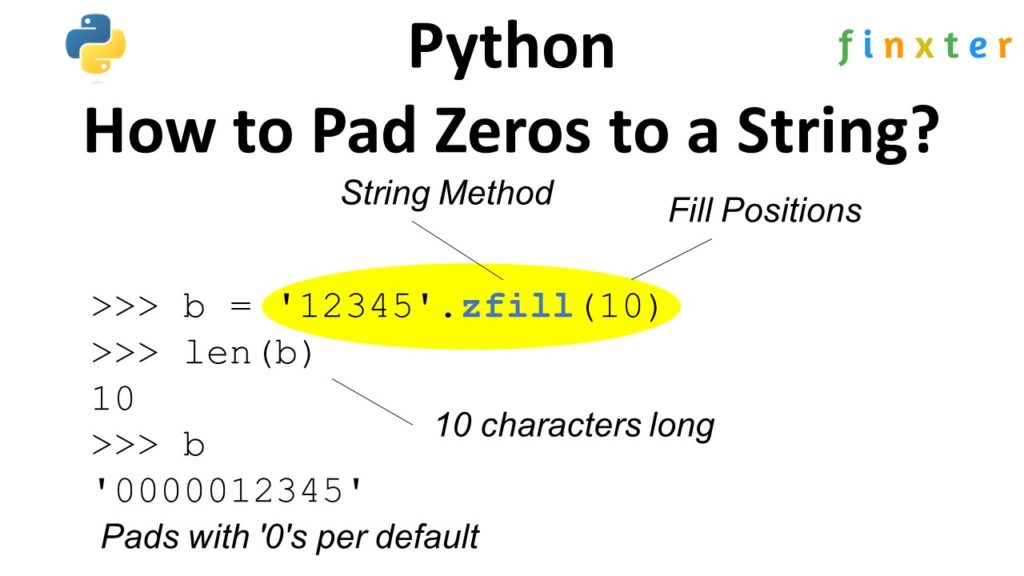
To convert an integer i to a string with leading zeros so that it consists of 5 characters, use the format string f'{i:05d}'. The d flag in this expression defines that the result is a decimal value. The str(i).zfill(5) accomplishes the same string conversion of an integer with leading zeros.
Challenge: Given an integer number. How to convert it to a string by adding leading zeros so that the string has a fixed number of positions.
Example: For integer 42, you want to fill it up with leading zeros to the following string with 5 characters: '00042'.
In all methods, we assume that the integer has less than 5 characters.
Method 1: Format String
The first method uses the format string feature in Python 3+. They’re also called replacement fields.
# Integer value to be converted
i = 42 # Method 1: Format String
s1 = f'{i:05d}'
print(s1)
# 00042
The code f'{i:05d}' places the integer i into the newly created string. However, it tells the format language to fill the string to 5 characters with leading '0's using the decimal system. This is the most Pythonic way to accomplish this challenge.
Method 2: zfill()
Another readable and Pythonic way to fill the string with leading 0s is the string.zfill() method.
The method takes one argument and that is the number of positions of the resulting string. Per default, it fills with 0s.
You can check out the following video tutorial from Finxter Adam:
Method 3: List Comprehension
Many Python coders don’t quite get the f-strings and the zfill() method shown in methods 2 and 3. If you don’t have time learning them, you can also use a more standard way based on string concatenation and list comprehension.
# Method 3: List Comprehension
s3 = str(i)
n = len(s3)
s3 = '0' * (5-len(s3)) + s3
print(s3)
You first convert the integer to a basic string. Then, you create the prefix of 0s you need to fill it up to n=5 characters and concatenate it to the integer’s string representation. The asterisk operator creates a string of 5-len(s3) zeros here.
Where to Go From Here?
Enough theory, let’s get some practice!
To become successful in coding, you need to get out there and solve real problems for real people. That’s how you can become a six-figure earner easily. And that’s how you polish the skills you really need in practice. After all, what’s the use of learning theory that nobody ever needs?
Practice projects is how you sharpen your saw in coding!
Do you want to become a code master by focusing on practical code projects that actually earn you money and solve problems for people?
Then become a Python freelance developer! It’s the best way of approaching the task of improving your Python skills—even if you are a complete beginner.
So, can you use a function with or without return value as an expression inside a list comprehension?
Answer: You can use any expression inside the list comprehension, including functions and methods. An expression can be an integer 42, a numerical computation 2+2 (=4), or even a function call np.sum(x) on any iterable x. Any function without return value, returns None per default. That’s why you can even call functions with side effects within a list comprehension statement.
Here’s an example:
[print('hi') for _ in range(10)] '''
hi
hi
hi
hi
hi
hi
hi
hi
hi
hi '''
You use the throw-away underscore _ because you want to execute the same function ten times. If you want to print the first 10 numbers to the shell, the following code does the trick:
[print(i) for i in range(10)] '''
0
1
2
3
4
5
6
7
8
9 '''
Let’s have a look at the content of the list you just created:
lst = [print(i) for i in range(10)]
print(lst)
# [None, None, None, None, None, None, None, None, None, None]
The list contains ten None values because the return value of the print() function is None. The side effect of executing the print function within the list comprehension statement is that the first ten values from 0 to 9 appear on your standard output.
Walrus Operator
Python 3.8 has introduced the walrus operator, also known as the assignment expression. This operator is useful if executing a certain function has side effects that you don’t want. For example, if you have a string creation method inside the list comprehension statement, conditioned by some filtering criterion in the if suffix. Without the walrus operator, Python would execute this same routine multiple times—even though this is highly redundant. You can avoid this redundancy by assigning it to a variable s once using the walrus operator and reusing this exact variable in the expression.
import random def get_random_string(): return f'sss {random.randrange(0, 100)}' # Goal: Print all random strings that contain 42 # WRONG
lst = [get_random_string() for _ in range(1000) if '42' in get_random_string()]
print(lst)
# ['sss 74', 'sss 13', 'sss 76', 'sss 13', 'sss 92', 'sss 96', 'sss 27', 'sss 43', 'sss 80'] # CORRECT
lst = [s for _ in range(1000) if '42' in (s := get_random_string())]
print(lst)
# ['sss 42', 'sss 42', 'sss 42', 'sss 42', 'sss 42', 'sss 42', 'sss 42', 'sss 42', 'sss 42', 'sss 42', 'sss 42', 'sss 42', 'sss 42']
With the walrus operator s := get_random_string(), you store the result of the function call in the variable s and retrieve it inside the expression part of the list comprehension. All of this happens inside the list comprehension statement.
I teach these concepts in my exclusive FINXTER email academy—join us, it’s free!
In Python’s pandas module, DataFrames are two-dimensional data objects. You can think of them as tables with rows and columns that contain data. This article provides an overview of the most common ways to instantiate DataFrames. We follow the convention to rename the pandas import to pd.
Create a DataFrame From a CSV File
Creating DataFrames with the function pd.read_csv(filename) is probably the best known. The first line of the csv file contains the column labels separated by commas. In the following lines follow the data points, in each row as many as there are columns. The data points must be separated by commas, if you want to use the default settings of pd.read_csv(). Here is an example of such a csv file:
The following code snippet creates a DataFrame from the data.csv file:
import pandas as pd df = pd.read_csv('data.csv')
The function pd.read_table() is similar but expects tabs as delimiters instead of comas. The default behavior of pandas adds an integer row index, yet it is also possible to choose one of the data columns to become the index column. To do so, use the parameter index_col. Example: pd.read_csv(‘data.csv’, index_col=0)
Create a DataFrame From a List of Lists
A DataFrame can be created from a list of lists where each list in the outer list contains the data for one row. To create the DataFrame we use the DataFrame’s constructor to which we pass the list of list and a list with the column labels:
import pandas as pd data = [ ['Bob', 23], ['Carl', 34], ['Dan', 14]
]
df = pd.DataFrame(data, columns=['Name', 'Age'])
Create a DataFrame From a Dictionary of Lists
A DataFrame can be created from a dictionary of lists. The dictionary’s keys are the column labels, the lists contain the data for the columns.
import pandas as pd # columns
names = ['Alice', 'Bob', 'Carl']
ages = [21, 27, 35] # create the dictionary of lists
data = {'Name':names, 'Age':ages} df = pd.DataFrame(data)
Create a DataFrame From a List of Dictionaries
A DataFrame can be created from a list of dictionaries. Each dictionary represents a row in the DataFrame. The keys in the dictionaries are the column labels and the values are the values for the columns.
The DataFrame constructor can also be called with a list of tuples where each tuple represents a row in the DataFrame. In addition we pass a list of column labels to the parameter columns.
import pandas as pd names = ['Alice', 'Bob', 'Clarisse', 'Dagobert']
ages = [20, 53, 42, 23] # create a list of tuples
data = list(zip(names, ages)) df = pd.DataFrame(data, columns=['Name', 'Age'])
Summing Up
In this article we have gone through a range of different ways to create DataFrames in pandas. However, it is not exhaustive. You should choose the method which best fits your use-case, this is to say, the method which requires the least amount of data transformation.
You’re not alone—thousands of coders like you generate this error in thousands of projects every single month. This short tutorial will show you exactly why this error occurs, how to fix it, and how to never make the same mistake again. So, let’s get started!
Python throws the TypeError object is not subscriptable if you use indexing with the square bracket notation on an object that is not indexable. This is the case if the object doesn’t define the __getitem__() method. You can fix it by removing the indexing call or defining the __getitem__ method.
The following code snippet shows the minimal example that leads to the error:
variable = None
print(variable[0])
# TypeError: 'NoneType' object is not subscriptable
You set the variable to the value None. The value None is not a container object, it doesn’t contain other objects. So, the code really doesn’t make any sense—which result do you expect from the indexing operation?
Exercise: Before I show you how to fix it, try to resolve the error yourself in the following interactive shell:
If you struggle with indexing in Python, have a look at the following articles on the Finxter blog—especially the third!
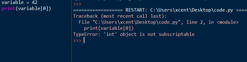
Note that a similar problem arises if you set the variable to the integer value 42 instead of the None value. The only difference is that the error message now is "TypeError: 'int' object is not subscriptable".
You can fix the non-subscriptable TypeError by wrapping the non-indexable values into a container data type such as a list in Python:
variable = [None]
print(variable[0])
# None
The output now is the value None and the script doesn’t throw an error anymore.
An alternative is to define the __getitem__ method in your code:
class X: def __getitem__(self, i): return f"Value {i}" variable = X()
print(variable[0])
# Value 0
You overwrite the __getitem__ method that takes one (index) argument i (in addition to the obligatory self argument) and returns the i-th value of the “container”. In our case, we just return a string "Value 0" for the element variable[0] and "Value 10" for the element variable[10]. It doesn’t make a lot of sense here but is the minimal example that shows how it works.
I hope you’d be able to fix the bug in your code! Before you go, check out our free Python cheat sheets that’ll teach you the basics in Python in minimal time:
The most Pythonic way to convert a list of floats fs to a list of integers is to use the one-liner fs = [int(x) for x in fs]. It iterates over all elements in the list fs using list comprehension and converts each list element x to an integer value using the int(x) constructor.
This article shows you the simplest ways to convert a one-dimensional list consisting only of floats to a list of int.
Problem: Given a list of floats [1.0, 2.0, 3.0]. How to convert it to a list of ints [1, 2, 3]?
The methods are not applicable to lists of lists, they contain rounding errors that are different in each method. If necessary, you can add cycles or define custom functions to check, account for and minimize errors.
Method 1: List Comprehension
Suppose we have a list:
a = [1.1, 1.2, 1.8, 0.5, 5.9, -2.3]
Now, check the type of the list numbers:
print(type(a[0]))
# <class 'float'>
Let’s apply the built-in function int, and get a list of integers:
print([int(a) for a in a])
# [1, 1, 1, 0, 5, -2]
Check the type of numbers in the new list:
A = [int(a) for a in a]
print(type(A[0]))
# <class ‘int’>
Thus, using the built-in function int, which converts a real number rounds towards zero, or rather, it discards the fractional part, we can get a new list of integers with a one-line code.
Method 2: Map Function
The built-in function map is well optimized and efficient, when it is called, the elements of the list are retrieved upon access. Therefore, one element is stored and processed in memory, which allows the program not to store the entire list of elements in the system memory.
Apply to the same list a the following code:
print(list(map(int, a)))
# [1, 1, 1, 0, 5, -2]
It makes no sense to check the type of the elements of the resulting list, since when we called the map function, we passed the int function already described in method 1 as an argument, and wrapped the result in a list using the list function.
The quality of this transformation of the list, or rather the rounding error, is the same as in the first method.
Method 3: Round & List Comprehension
It is very similar to the first, but unlike int, it doesn’t just discard the fractional part but rounds to the nearest even integer if the fractional part is 0.5. You can also pass as the second argument the number of decimal places to which rounding is required, by default it is 0, this is what we will use:
print([round(a) for a in a])
Check the type of numbers in the new list:
D = [round(a) for a in a]
print(type(D[0]))
# <class ‘int’>
As you can see from this example, there are different built-in functions to achieve our goal, the difference is in the method and the magnitude of the rounding error.
Method 4: Math Module
In this way, I suggest using the imported module math, in which we will use the three functions ceil(), floor(), and trunc(). let’s take a closer look at each. They have the same syntax, the difference is in the way of rounding.
Let’s apply to the original list:
a = [1.1, 1.2, 1.8, 0.5, 5.9, -2.3]
print([math.ceil(a) for a in a])
# [2, 2, 2, 1, 6, -2]
‘Ceil’ rounds to the next largest integer, respecting the sign(-2.3 < -2 which is True).
Check the type of numbers in the new list:
C = [math.ceil(a) for a in a]
print(type(C[0]))
# <class ‘int’>
Consider the following function in the ‘math’ – ‘floor’ module, which is the opposite of ‘ceil’ – rounding down to the nearest integer:
print([math.floor(a) for a in a])
# [1, 1, 1, 0, 5, -3]
Check the type:
F = [math.floor(a) for a in a]
print(type(F[0]))
# <class ‘int’>
The next function, trunc(), is analogous to the built-in function int() — it simply discards the fractional part whatever it is:
print([math.trunc(a) for a in a])
# [1, 1, 1, 0, 5, -2]
And check the type:
T = [math.trunc(a) for a in a]
print(type(T[0]))
# <class ‘int’>
Method 5: NumPy
Here’s a look at converting a list from an int to an array using the NumPy module. The difference between an array and a list is that all elements of an array must be of the same type, like “float” and “int”. Numeric operations with large amounts of data can be performed with arrays much faster and more efficiently than with lists.
Let’s turn our first list a into an array:
import numpy as np
N = np.array(a, int)
We pass two arguments to the array function, the name of the list to convert to an array and the type for each element.
# [ 1 1 1 0 5 -2]
Сheck the type of elements:
print(type(N[0]))
# <class 'numpy.int32'>
Unlike the int number type in Python, the NumPy module defines them slightly differently and is divided into several subgroups. For example, 'int32' are integers ranging from -2147483648 to 2147483647 (4-byte numbers), 'int64' are numbers from -9223372036854775808 to 9223372036854775807 (8-byte numbers), there are also different types of 'int' for 32- and 64-bit operating systems, this must be taken into account when calculating with arrays.
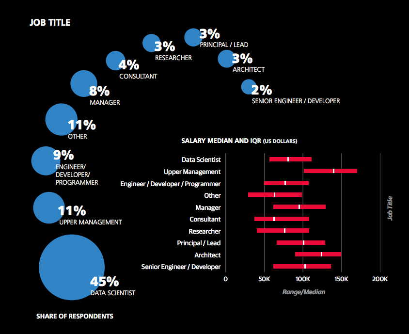
A recent study from O’Reilly found that data science is a wide field with many specializations and job descriptions. However, the average earning of an employed data scientist—45% of all respondents would consider themselves as such—is between $60,000 and $110,000. This means that experienced data scientists over time quite certainly reach six-figure income levels if they keep improving and searching for new opportunities. Here’s a screenshot from the report showing the different routes you can go:
You can see that there are significant opportunities “down the line” by working as an architect, team leader, or manager that earn significantly above six-figures. Becoming an employed data scientist remains an attractive way to make a great living.
But what about freelance data scientists? Do they earn more?
The best data comes directly from the source: Upwork, the biggest freelancer market in the world. Let’s dive into some profiles from freelance data scientists!
Here’s a table of 24 freelance data scientists incomes from the Upwork results:
Freelancer
Hourly Income
Earned
Job Success
Data Science & Machine Learning
$60
$100.000
100%
Data Science & Machine Learning
$300
$100.000
100%
Data Science Consultant
$50
$10.000
97%
Data Science & Machine Learning
$25
$10.000
91%
Data Science/Analyst, Statistician
$70
$100.000
97%
Applied Machine Learning
$300
$50.000
100%
Chief Technology Officer
$55
$200.000
100%
Computer Vision
$32
$2.000.000
100%
Data Engineer
$50
$10.000
100%
Research Scientist
$150
$700.000
95%
Analytics Expert
$52
$10.000
100%
Deep Learning Expert
$195
$10.000
100%
Data Scientist
$60
$10.000
77%
Scalable Analytics Consultant
$300
$500.000
100%
Machine Learning
$40
$8.000
91%
Machine Learning
$80
$30.000
100%
Tutor
$30
$20.000
92%
Math
$38
$4.000
100%
NLP
$35
$30.000
71%
Machine Learning
$50
$4.000
100%
Big Data Engineer
$50
$10.000
100%
AVERAGE
$96
$186.476
96%
The tabular data is drawn from 100 Upwork freelancer profiles as they appeared in the Upwork search. We randomly chose profiles and filtered them for data availability (e.g., total money earned). The result is that the average freelance data scientist earns $96 per hour. For 1700 working hours per year and a full schedule, this results in an average annual income of $163,200. To accomplish this, you need to join the ranks of relatively high-rated freelancers above 90% job satisfaction.
Let’s have a look at some other data sources: As a data scientist, you’re a programmer—in a way. The demand for programming talent has steadily increased in the preceding decades.
Here’s a quick tabular overview of what you can earn as a data scientist—it shows that as a data scientist, you’re in effect a well-compensated coder with specific skill sets.
Title
Best Programming Languages
Yearly Income (Average US)
Web Developer
JavaScript + HTML + CSS + SQL
$78,088
Mobile Developer Android
Java
$126,154
Mobile Developer Apple
Swift
$123,263
Back End Developer
Python + Django + Flask
$127,913
Front End Developer
JavaScript + HTML + CSS
$109,742
Full-Stack Engineer
Python + JavaScript + HTML + CSS + SQL
$112,098
Data Scientist
Python + Matplotlib + Pandas + NumPy + Dash
$122,700
Machine Learning Engineer
Python + NumPy + Scikit-Learn + TensorFlow
$145,734
Let’s dive into the different freelance developer career choices for maximum success!
Do you want to develop the skills of a well-rounded Python professional—while getting paid in the process? Become a Python freelancer and order your book Leaving the Rat Race with Python on Amazon (Kindle/Print)!
Where to Go From Here?
Enough theory, let’s get some practice!
To become successful in coding, you need to get out there and solve real problems for real people. That’s how you can become a six-figure earner easily. And that’s how you polish the skills you really need in practice. After all, what’s the use of learning theory that nobody ever needs?
Practice projects is how you sharpen your saw in coding!
Do you want to become a code master by focusing on practical code projects that actually earn you money and solve problems for people?
Then become a Python freelance developer! It’s the best way of approaching the task of improving your Python skills—even if you are a complete beginner.