Python’s built-in abs(x) function returns the absolute value of the argument x that can be an integer, float, or object implementing the __abs__() function. For a complex number, the function returns its magnitude. The absolute value of any numerical input argument -x or +x is the corresponding positive value +x.

Argument	x	int, float, complex, object with __abs__() implementation
Return Value	|x|	Returns the absolute value of the input argument. Integer input –> Integer output Float input –> Float output Complex input –> Complex output

Interactive Code Shell

Example Integer abs()

The following code snippet shows you how to use the absolute value 42 of a positive integer value 42.

# POSITIVE INTEGER
x = 42
abs_x = abs(x) print(f"Absolute value of {x} is {abs_x}")
# Absolute value of 42 is 42

The following code snippet shows you how to use the absolute value 42 of a negative integer value -42.

# NEGATIVE INTEGER
x = -42
abs_x = abs(x) print(f"Absolute value of {x} is {abs_x}")
# Absolute value of -42 is 42

Example Float abs()

The following code snippet shows you how to use the absolute value 42.42 of a positive integer value 42.42.

# POSITIVE FLOAT
x = 42.42
abs_x = abs(x) print(f"Absolute value of {x} is {abs_x}")
# Absolute value of 42.42 is 42.42

The following code snippet shows you how to use the absolute value 42.42 of a negative integer value -42.42.

# NEGATIVE FLOAT
x = -42.42
abs_x = abs(x) print(f"Absolute value of {x} is {abs_x}")
# Absolute value of -42.42 is 42.42

Example Complex abs()

The following code snippet shows you how to use the absolute value of a complex number (3+10j).

# COMPLEX NUMBER
complex_number = (3+10j)
abs_complex_number = abs(complex_number) print(f"Absolute value of {complex_number} is {abs_complex_number}")
# Absolute value of (3+10j) is 10.44030650891055

Python abs() vs fabs()

Python’s built-in function abs(x) calculates the absolute number of the argument x. Similarly, the fabs(x) function of the math module calculates the same absolute value. The difference is that math.fabs(x) always returns a float number while Python’s built-in abs(x) returns an integer if the argument x is an integer as well. The name “fabs” is shorthand for “float absolute value”.

Here’s a minimal example:

x = 42 # abs()
print(abs(x))
# 42 # math.fabs()
import math
print(math.fabs(x))
# 42.0

Python abs() vs np.abs()

Python’s built-in function abs(x) calculates the absolute number of the argument x. Similarly, NumPy’s np.abs(x) function calculates the same absolute value. There are two differences: (1) np.abs(x) always returns a float number while Python’s built-in abs(x) returns an integer if the argument x is an integer, and (2) np.abs(arr) can be also applied to a NumPy array arr that calculates the absolute values element-wise.

Here’s a minimal example:

x = 42 # abs()
print(abs(x))
# 42 # numpy.abs()
import numpy as np
print(np.fabs(x))
# 42.0 # numpy.abs() array
a = np.array([-1, 2, -4])
print(np.abs(a))
# [1 2 4]

abs and np. absolute are completely identical. It doesn’t matter which one you use. There are several advantages to the short names: They are shorter and they are known to Python programmers because the names are identical to the built-in Python functions.

Summary

The abs() function is a built-in function that returns the absolute value of a number. The function accepts integers, floats, and complex numbers as input.

If you pass abs() an integer or float, n, it returns the non-negative value of n and preserves its type. In other words, if you pass an integer, abs() returns an integer, and if you pass a float, it returns a float.

# Int returns int
>>> abs(20)
20
# Float returns float
>>> abs(20.0)
20.0
>>> abs(-20.0)
20.0

The first example returns an int, the second returns a float, and the final example returns a float and demonstrates that abs() always returns a positive number.

Complex numbers are made up of two parts and can be written as a + bj where a and b are either ints or floats. The absolute value of a + bj is defined mathematically as math.sqrt(a**2 + b**2). Thus, the result is always positive and always a float (since taking the square root always returns a float).

>>> abs(3 + 4j)
5.0
>>> math.sqrt(3**2 + 4**2)
5.0

Here you can see that abs() always returns a float and that the result of abs(a + bj) is the same as math.sqrt(a**2 + b**2).

Where to Go From Here?

Enough theory, let’s get some practice!

To become successful in coding, you need to get out there and solve real problems for real people. That’s how you can become a six-figure earner easily. And that’s how you polish the skills you really need in practice. After all, what’s the use of learning theory that nobody ever needs?

Practice projects is how you sharpen your saw in coding!

Do you want to become a code master by focusing on practical code projects that actually earn you money and solve problems for people?

Then become a Python freelance developer! It’s the best way of approaching the task of improving your Python skills—even if you are a complete beginner.

Join my free webinar “How to Build Your High-Income Skill Python” and watch how I grew my coding business online and how you can, too—from the comfort of your own home.

Join the free webinar now!

The post Python abs() Function first appeared on Finxter.

Python comes with many built-in functions you can use without importing any library. Here are they in alphabetical order:

		Built-in Functions
abs()	delattr()	hash()	memoryview()	set()
all()	dict()	help()	min()	setattr()
any()	dir()	hex()	next()	slice()
ascii()	divmod()	id()	object()	sorted()
bin()	enumerate()	input()	oct()	staticmethod()
bool()	eval()	int()	open()	str()
breakpoint()	exec()	isinstance()	ord()	sum()
bytearray()	filter()	issubclass()	pow()	super()
bytes()	float()	iter()	print()	tuple()
callable()	format()	len()	property()	type()
chr()	frozenset()	list()	range()	vars()
classmethod()	getattr()	locals()	repr()	zip()
compile()	globals()	map()	reversed()	__import__()
complex()	hasattr()	max()	round()

The post Python Built-In Functions first appeared on Finxter.

In this article, you’ll explore how to generate exponential fits by exploiting the curve_fit() function from the Scipy library. SciPy’s curve_fit() allows building custom fit functions with which we can describe data points that follow an exponential trend.

• In the first part of the article, the curve_fit() function is used to fit the exponential trend of the number of COVID-19 cases registered in California (CA).
• The second part of the article deals with fitting histograms, characterized, also in this case, by an exponential trend.

Disclaimer: I’m not a virologist, I suppose that the fitting of a viral infection is defined by more complicated and accurate models; however, the only aim of this article is to show how to apply an exponential fit to model (to a certain degree of approximation) the increase in the total infection cases from the COVID-19. 

Exponential fit of COVID-19 total cases in California

Data related to the COVID-19 pandemic have been obtained from the official website of the “Centers for Disease Control and Prevention” (https://data.cdc.gov/Case-Surveillance/United-States-COVID-19-Cases-and-Deaths-by-State-o/9mfq-cb36) and downloaded as a .csv file. The first thing to do is to import the data into a Pandas dataframe. To do this, the Pandas functions pandas.read_csv() and pandas.Dataframe() were employed. The created dataframe is made up of 15 columns, among which we can find the submission_date, the state, the total cases, the confirmed cases and other related observables. To gain an insight into the order in which these categories are displayed, we print the header of the dataframe; as can be noticed, the total cases are listed under the voice “tot_cases”.

Since in this article we are only interested in the data related to the California, we create a sub-dataframe that contains only the information related to the California state. To do that, we exploit the potential of Pandas in indexing subsections of a dataframe. This dataframe will be called df_CA (from California) and contains all the elements of the main dataframe for which the column “state” is equal to “CA”. After this step, we can build two arrays, one (called tot_cases) that contains the total cases (the name of the respective header column is “tot_cases”) and one that contains the number of days passed by the first recording (called days). Since the data were recorded daily, in order to build the “days” array, we simply build an array of equally spaced integer number from 0 to the length of the “tot_cases” array, in this way, each number refers to the n° of days passed from the first recording (day 0).

At this point, we can define the function that will be used by curve_fit() to fit the created dataset. An exponential function is defined by the equation:

y = a*exp(b*x) +c

where a, b and c are the fitting parameters. We will hence define the function exp_fit() which return the exponential function, y, previously defined. The curve_fit() function takes as necessary input the fitting function that we want to fit the data with, the x and y arrays in which are stored the values of the datapoints. It is also possible to provide initial guesses for each of the fitting parameters by inserting them in a list called p0 = […] and upper and lower boundaries for these parameters (for a comprehensive description of the curve_fit() function, please refer to https://docs.scipy.org/doc/scipy/reference/generated/scipy.optimize.curve_fit.html ). In this example, we will only provide initial guesses for our fitting parameters. Moreover, we will only fit the total cases of the first 200 days; this is because for the successive days, the number of cases didn’t follow an exponential trend anymore (possibly due to a decrease in the number of new cases). To refer only to the first 200 values of the arrays “days” and “tot_cases”, we exploit array slicing (e.g. days[:200]).

The output of curve_fit() are the fitting parameters, presented in the same order that was used during their definition, within the fitting function. Keeping this in mind, we can build the array that contains the fitted results, calling it “fit_eq”.

Now that we built the fitting array, we can plot both the original data points and their exponential fit.

The final result will be a plot like the one in Figure 1:

Application of an exponential fit to histograms

Now that we know how to define and use an exponential fit, we will see how to apply it to the data displayed on a histogram. Histograms are frequently used to display the distributions of specific quantities like prices, heights etc…The most common type of distribution is the Gaussian distribution; however, some types of observables can be defined by a decaying exponential distribution. In a decaying exponential distribution, the frequency of the observables decreases following an exponential[A1]  trend; a possible example is the amount of time that the battery of your car will last (i.e. the probability of having a battery lasting for long periods decreases exponentially). The exponentially decaying array will be defined by exploiting the Numpy function random.exponential(). According to the Numpy documentation, the random.exponential() function draws samples from an exponential distribution; it takes two inputs, the “scale” which is a parameter defining the exponential decay and the “size” which is the length of the array that will be generated. Once obtained random values from an exponential distribution, we have to generate the histogram; to do this, we employ another Numpy function, called histogram(), which generates an histogram taking as input the distribution of the data (we set the binning to “auto”, in this way the width of the bins is automatically computed). The output of histogram() is a 2D array; the first array contains the  frequencies of the distribution while the second one contains the edges of the bins. Since we are only interested in the frequencies, we assign the first output to the variable “hist”. For this example, we will generate the array containing the bin position by using the Numpy arange() function; the bins will have a width of 1 and their number will be equal to the number of elements contained in the “hist” array.

At this point, we have to define the fitting function and to call curve_fit() for the values of the just created histogram. The equation describing an exponential decay is similar to the one defined in the first part; the only difference is that the exponent has a negative sign, this allows the values to decrease according to an exponential fashion. Since the elements in the “x” array, defined for the bin position, are the coordinates of the left edge of each bin, we define another x array that stores the position of the center of each bin (called “x_fit”); this allows the fitting curve to pass through the center of each bin, leading to a better visual impression. This array will be defined by taking the values of the left side of the bins (“x” array elements) and adding half the bin size; which corresponds to half the value of the second bin position (element of index 1). Similar to the previous part, we now call curve_fit(), generate the fitting array and assign it to the varaible “fit_eq”.

Once the distribution has been fitted, the last thing to do is to check the result by plotting both the histogram and the fitting function. In order to plot the histogram, we will use the matplotlib function bar(), while the fitting function will be plotted using the classical plot() function.

The final result is displayed in Figure 2:

Summary

In these two examples, the curve_fit() function was used to apply to different exponential fits to specific data points. However, the power of the curve_fit() function, is that it allows you defining your own custom fit functions, being them linear, polynomial or logarithmic functions. The procedure is identical to the one shown in this article, the only difference is in the shape of the function that you have to define before calling curve_fit().

---

Full Code

import pandas as pd
import numpy as np
import matplotlib.pyplot as plt
from scipy.optimize import curve_fit url = "United_States_COVID-19_Cases_and_Deaths_by_State_over_Time" #url of the .csv file
file = pd.read_csv(url, sep = ';', thousands = ',') # import the .csv file
df = pd.DataFrame(file) # build up the pandas dataframe
print(df.columns) #visualize the header
df_CA = df[df['state'] == 'CA'] #initialize a sub-dataframe for storing only the values for the California
tot_cases = np.array((df_CA['tot_cases'])) #create an array with the total n° of cases
days = np.linspace(0, len(tot_cases), len(tot_cases)) # array containing the n° of days from the first recording #DEFINITION OF THE FITTING FUNCTION
def exp_fit(x, a, b, c): y = a*np.exp(b*x) + c return y #----CALL THE FITTING FUNCTION----
fit = curve_fit(exp_fit,days[:200],tot_cases[:200], p0 = [0.005, 0.03, 5])
fit_eq = fit[0][0]*np.exp(fit[0][1]*days[:200])+fit[0][2] # #----PLOTTING-------
fig = plt.figure()
ax = fig.subplots()
ax.scatter(days[:200], tot_cases[:200], color = 'b', s = 5)
ax.plot(days[:200], fit_eq, color = 'r', alpha = 0.7)
ax.set_ylabel('Total cases')
ax.set_xlabel('N° of days')
plt.show() #-----APPLY AN EXPONENTIAL FIT TO A HISTOGRAM--------
data = np.random.exponential(5, size=10000) #generating a random exponential distribution
hist = np.histogram(data, bins="auto")[0] #generating a histogram from the exponential distribution
x = np.arange(0, len(hist), 1) # generating an array that contains the coordinated of the left edge of each bar #---DECAYING FIT OF THE DISTRIBUTION----
def exp_fit(x,a,b): #defining a decaying exponential function y = a*np.exp(-b*x) return y x_fit = x + x[1]/2 # the point of the fit will be positioned at the center of the bins
fit_ = curve_fit(exp_fit,x_fit,hist) # calling the fit function
fit_eq = fit_[0][0]*np.exp(-fit_[0][1]*x_fit) # building the y-array of the fit
#Plotting
plt.bar(x,hist, alpha = 0.5, align = 'edge', width = 1)
plt.plot(x_fit,fit_eq, color = 'red')
plt.show()

The post Exponential Fit with SciPy’s curve_fit() first appeared on Finxter.

This tutorial taken from my upcoming programming book “From One to Zero” (NoStarch, 2021) will show you how to write great comments. While most online tutorials focus on a bullet list of commenting tips, we dive deeper into the meat exploring the underlying reasons for the commonly recommended commenting principles. So, let’s get started!

Code For Humans Not Machines

“Any fool can write code that a computer can understand. Good programmers write code that humans can understand.” — Martin Fowler

The main purpose of source code is to define what machines should do and how to do it.

Yet, if this was the only criteria, you’d use a low-level machine language such as assembler to accomplish this goal because it’s the most expressive and most powerful language.

The purpose of high-level programming languages such as Python is to help people write better code and do it more quickly. Our next principle for clean code is to constantly remind yourself that you’re writing code for other people and not for machines.

If your code will have any impact in the real world, it’ll be read multiple times by you or a programmer that takes your place if you stop working on the code base. Always assume that your source code will be read by other people. What can you do to make their job easier? Or, to put it more plainly: what can you do to mitigate the negative emotions they’ll experience against the original programmer of the code base their working on? Code for people not machines!

Reduce Time to Understanding

If you write code for humans not machines, you’ll need to use comments to help readers of your code understand it better and quicker. A short comment can greatly reduce the time to cognitively grasp the meaning of the code base. Consider the following code example:

import re text = ''' Ha! let me see her: out, alas! he's cold: Her blood is settled, and her joints are stiff; Life and these lips have long been separated: Death lies on her like an untimely frost Upon the sweetest flower of all the field. ''' f_words = re.findall('\\bf\w+\\b', text)
print(f_words) l_words = re.findall('\\bl\w+\\b', text)
print(l_words) '''
OUTPUT:
['frost', 'flower', 'field']
['let', 'lips', 'long', 'lies', 'like'] '''

Bad code example without comments.

The previous code snippet analyzes a short text snippet from Shakespeare’s Romeo and Juliet using regular expressions. If you’re not very familiar with regular expressions, you probably struggle understanding what the code does. Even the meaningful variable names don’t help much. Let’s see if a few comments can resolve your confusion!

import re text = ''' Ha! let me see her: out, alas! he's cold: Her blood is settled, and her joints are stiff; Life and these lips have long been separated: Death lies on her like an untimely frost Upon the sweetest flower of all the field. ''' # Find all words starting with character 'f'
f_words = re.findall('\\bf\w+\\b', text)
print(f_words) # Find all words starting with character 'l'
l_words = re.findall('\\bl\w+\\b', text)
print(l_words) '''
OUTPUT:
['frost', 'flower', 'field']
['let', 'lips', 'long', 'lies', 'like'] '''

Good code example with comments.

The two short comments greatly help understanding the regular expression patterns '\\bf\w+\\b' and '\\bl\w+\\b'. While I won’t dive deeply into regular expressions here, the example shows how comments can help you getting a rough understanding of other people’s code without understanding each and every syntactic sugar. For introductory tutorials into the powerful technology regular expressions, check out our two technical books Python One-Liners and The Smartest Way to Learn Python Regular Expressions.

You’re the Expert—Share Your Wisdom!

Helpful comments give a glimpse into your thinking—as you’ve written the code, you possess valuable insight into it only matched by very few persons. Don’t miss out on sharing your insights with other people! Comments can be very useful to “abstract” over blocks of code. For example, if you have five lines of code dealing with updating customer information in a database, add a short comment before the block to explain this. This will help the reader get a quick overview of your code and accelerates their and your “code loading time”. You can find an example of such an instance next:

# Process next order
order = get_next_order()
user = order.get_user()
database.update_user(user)
database.update_product(order.get_order()) # Ship order & confirm customer
logistics.ship(order, user.get_address())
user.send_confirmation()

Commented blocks help get an overview of the code.

The code exemplifies how an online shop completes a customer order in two high-level steps: (1) Processing the next order, and (2) Shipping the order. The comments help you understand the purpose of the code in a few seconds without the need to look at each individual method call.  

Comments as WARNINGS!

You can also use comments as a warning of potentially undesired consequences. This increases the level of attention of the programmer working with your code. The following code shows such an example where programmers are warned before calling a function ship_yacht() that will actua ship an expensive yacht to a customer.

##########################################################
# WARNING #
# EXECUTING THIS FUNCTION WILL SHIP A $1,569,420 YACHT!! #
##########################################################
def ship_yacht(customer): database.update(customer.get_address()) logistics.ship_yacht(customer.get_address()) logistics.send_confirmation(customer)

Comments as warnings.

There are many more ways to use comments in a useful way. Comments are always there for the human reader, so always keep in mind that you’re writing code for humans not machines!

Avoid Unnecessary Comments

Not all comments help readers understand code better. In fact, there are many cases where comments reduce the clarity and confuse the readers of a given code base. If your goal is to write clean code, you must not only use valuable comments but also avoid unnecessary comments. But what are unnecessary comments? Let’s dive into those next.

During my time as a computer science researcher, many of my senior-level students described me in great detail how their job interviews at various companies went. A very skilled student had successfully applied for a job at Google. He told me that the Google headhunters—they’re usually Google engineers—criticized his code style because he added too many unnecessary comments. These types of comments are so called “code smells”—expert coders can figure out very quickly whether you’re a beginner, intermediate, or expert coder yourself. Unnecessary comments make this very obvious. But what are unnecessary comments? In most cases, they add a level of redundancy to the code. A great coder will use meaningful variable names (Principle: Use the Right Names), so the code often becomes self-explanatory—at least in comparison to code that doesn’t use the right names. Let’s revisit the code snippet with meaningful variable names.

investments = 10000
yearly_return = 0.1
years = 10 for year in range(years): print(investments * (1 + yearly_return)**year)

No comments needed.

The code calculates your cumulative investment return for ten years assuming a 10% yield. Now, let’s add some unnecessary comments!

investments = 10000 # your investments, change if needed
yearly_return = 0.1 # annual return (e.g., 0.1 --> 10%)
years = 10 # number of years to compound # Go over each year
for year in range(years): # Print value of your investment in current year print(investments * (1 + yearly_return)**year)

Unnecessary comments.

All comments in the previous code snippet are redundant. Some of them would’ve been useful if you’d chosen less meaningful variable names such as x, y, or z. But explaining a variable named yearly_return by means of a comment doesn’t provide any relative value. Quite contrarily, it reduces the value because it adds unnecessary clutter to the code. The additional clutter makes your code less readable and less concise. There are a few rules that may help you avoid unnecessary comments—although the best rule is to use your common sense to identify whether a comment really improves the readability of your code.

Code Smells — Negative Commenting Principles

• Don’t use inline comments. They have little value and can be completely avoided by choosing meaningful variable names.
• Don’t be redundant. Redundancy is the enemy of clarity—this also holds for comments!
• Don’t add obvious comments. You can see an obvious comment in the previous code snippet just before the for loop statement. Any coder knows the for loop, so what additional value do you provide with the comment # Go over each year when the for loop already states for year in range(years)?  
• Don’t comment out code. If you’re a programmer, it’s very likely that you’ve been guilty of this. We programmers often hang on to our beloved code snippets even if we already (grudgingly) decided to remove them. The shy approach to removing unnecessary code is to comment it out. However, commented code is a readability killer and you should avoid it at all costs if you want to write clean code. Instead of commenting out the unnecessary code, boldly remove it. For your piece of mind, you should use a version history tool such as Git that allows you to get any old code snippet if you need it.

Many programming languages such as Python come with documentation functionality that allows you to describe the purpose of each function, method, and class in your code. If you’ve carefully chosen the abstraction level of each function (Single-Responsibility Principle), it’s often enough to use the build in documentation functionality instead of comments to describe what your code does. This largely removes the need for additional comments in your code.

---

Do you want to develop the skills of a well-rounded Python professional—while getting paid in the process? Become a Python freelancer and order your book Leaving the Rat Race with Python on Amazon (Kindle/Print)!

Where to Go From Here?

Enough theory, let’s get some practice!

To become successful in coding, you need to get out there and solve real problems for real people. That’s how you can become a six-figure earner easily. And that’s how you polish the skills you really need in practice. After all, what’s the use of learning theory that nobody ever needs?

Practice projects is how you sharpen your saw in coding!

Do you want to become a code master by focusing on practical code projects that actually earn you money and solve problems for people?

Then become a Python freelance developer! It’s the best way of approaching the task of improving your Python skills—even if you are a complete beginner.

Join my free webinar “How to Build Your High-Income Skill Python” and watch how I grew my coding business online and how you can, too—from the comfort of your own home.

Join the free webinar now!

The post Show Don’t Tell: Commenting Python Best Practices first appeared on Finxter.

This chapter draft from my upcoming book From One to Zero to appear in 2021 with NoStarch will teach you why and how to write clean and simple code. To stay tuned about the book release, sign up for the Finxter email coding acadamy (it’s free)!

---

Write Clean & Simple Code

Story: I learned to focus on writing clean code the hard way. One of my research projects during my time as a doctoral researcher in distributed systems was to code a distributed graph processing system from scratch. The system allowed you to run graph algorithms such as computing the shortest path on a large map in a distributed environment to speed up computation among multiple machines. If you’ve ever written a distributed application where two processes that reside on different computers interact with each other via messages, you know that the complexity can quickly become overwhelming. My code had thousands of lines of code and bugs were popping up frequently. I didn’t make any progress for weeks at a time—it was very frustrating. In theory, the concepts I developed sounded great and convincing. But practice got me! Finally, after a month or so working full-time on the code base without seeing any encouraging progress, I decided to radically simplify the code base. I started to use libraries instead of coding functions myself. I removed large code blocks of premature optimizations (see later). I removed code blocks that I had commented out for a possible later use. I refactored variable and function names. I structured the code in logical units and classes. And, after a week or so, not only was my code more readable and understandable by other researchers, it was also more efficient and less buggy. I managed to make progress again and my frustration quickly morphed into enthusiasm—clean code had rescued my research project!

Complexity: In the previous chapters, you’ve learned how harmful complexity is for any code project in the real world. Complexity kills your productivity, motivation, and time. Because most of us haven’t learned to speak in source code from an early age, it can quickly overwhelm our cognitive abilities. The more code you have, the more overwhelming it becomes. But even short code snippets and algorithms can be complicated. The following one-liner code snippet from our book Python One-Liners is a great example of a piece of source code that is short and concise, but still complex!

# Quicksort algorithm to sort a list of integers
unsorted = [33, 2, 3, 45, 6, 54, 33] q = lambda l: q([x for x in l[1:] if x <= l[0]]) + [l[0]] + q([x for x in l if x > l[0]]) if l else [] print(q(unsorted))
# [2, 3, 6, 33, 33, 45, 54]

You can find an explanation of this code snippet in our book Python One-Liners or online at https://blog.finxter.com/python-one-line-quicksort/.

Complexity comes from many directions when working with source code. It slows down our understanding of the code. And it increases the number of bugs in our code. Both slow understanding and more bugs increase the project costs and the number of people hours required to finish it. Robert C. Martin, author of the book Clean Code, argues that the more difficult it is to read and understand code, the higher the costs to write code as well:

“Indeed, the ratio of time spent reading versus writing is well over 10 to 1. We are constantly reading old code as part of the effort to write new code. …[Therefore,] making it easy to read makes it easier to write.” — Robert C. Martin

This relationship is visualized in Figure 5-1. The x axis corresponds to the number of lines written in a given code project. The y axis corresponds to the time to write one additional line of code. In general, the more code you’ve already written in one project, the more time it takes to write an additional line of code. Why is that? Say, you’ve written n lines of code and you add the n+1^st line of code. Adding this line may have an effect on potentially all previously written lines. It may have a small performance penalty which impacts the overall project. It may use a variable that is defined at another place. It may introduce a bug (with probability c) and to find that bug, you must search the whole project (so, your expected costs per line of code is c * T(n) for a steadily increasing function T with increasing input n). It may force you to write additional lines of code to ensure backward compatibility. There are many more reasons but you get the point: the additional complexity causes to slow down your progress the more code you’ve written.

Figure 5-1: Clean code improves scalability and maintainability of your code base.

But Figure 5-1 also shows the difference between writing dirty versus clean code. If writing dirty code wouldn’t result in any benefit, nobody would do it! There’s a very real benefit of writing dirty code: it’s less time consuming in the short-term and for small code projects. If you cram all the functionality in a 100-line code script, you don’t need to invest a lot of time thinking and structuring your project. But as you add more and more code, the monolithic code file grows from 100 to 1000 lines and at a certain point, it’ll be much less efficient compared to a more thoughtful approach where you structure the code logically in different modules, classes, or files.  As a rule of thumb: try to always write thoughtful and clean code—because the additional costs for thinking, refactoring, and restructuring will pay back many times over for any non-trivial project. Besides—writing clean code is just the right thing to do. The philosophy of carefully crafting your programming art will carry you further in life.

You don’t always know the second-order consequences of your code. Think of the spacecraft on a mission towards Venus in 1962 where a tiny bug—an omission of a hyphen in the source code—caused NASA engineers to issue a self-destruct command which resulted in a loss of the rocket worth more than $18 million at the time.

To mitigate all of those problems, there’s a simple solution: write simpler code. Simple code is less error-prone, less crowded, easier to grasp, and easier to maintain. It is more fun to read and write. In many cases, it’s more efficient and takes less space. It also facilitates scaling your project because people won’t be scared off by the complexity of the project. If new coders peek in your code project to see whether they want to contribute, they better believe that they can understand it. With simple code, everything in your project will get simpler. You’ll make faster progress, get more support, spend less time debugging, be more motivated, and have more fun in the process.

So, let’s learn how to write clean and simple code, shall we?

Clean code is elegant and pleasing to read. It is focused in the sense that each function, class, module focuses on one idea. A function transfer_funds(A,B) in your banking application does just that—transferring funds from account A to account B. It doesn’t check the credit of the sender A —for this, there’s another function check_credit(A). Simple but easy to understand and focused. How do you get simple and clean code? By spending time and effort to edit and revise the code. This is called refactoring and it must be a scheduled and crucial element of your software development process.

Let’s dive into some principles to write clean code. Revisit them from time to time—they’ll become meaningful sooner or later if you’re involved in some real-world projects.

Principles to Write Clean Code

Next, you’ll going to learn a number of principles that’ll help you write cleaner code.

Principle 1: You Ain’t Going to Need It

The principle suggests that you should never implement code if you only expect that you’re going to need its provided functionality someday in the future—because you ain’t gonna need it! Instead, write code only if you’re 100% sure that you need it. Code for today’s needs and not tomorrow’s.

It helps to think from first principles: The simplest and cleanest code is the empty file. It doesn’t have any bug and it’s easy to understand. Now, go from there—what do you need to add to that? In Chapter 4, you’ve learned about the minimum viable product. If you minimize the number of features you pursue, you’ll harvest cleaner and simpler code than you could ever attain through refactoring methods or all other principles combined. As you know by now, leaving out features is not only useful if they’re unnecessary. Leaving them out even makes sense if they provide relatively little value compared to other features you could implement instead. Opportunity costs are seldomly measured but most often they are very significant. Only because a feature provides some benefits doesn’t justify its implementation. You have to really need the feature before you even consider implementing it. Reap the low-hanging fruits first before you reach higher!

Principle 2: The Principle of Least Surprise

This principle is one of the golden rules of effective application and user experience design. If you open the Google search engine, the cursor will be already focused in the search input field so that you can start typing your search keyword right away without needing to click into the input field. Not surprising at all—but a great example of the principle of least surprise. Clean code also leverages this design principle. Say, you write a currency converter that converts the user’s input from USD to RMB. You store the user input in a variable. Which variable name is better suited, user_input or var_x? The principle of least surprise answers this question for you!

Principle 3: Don’t Repeat Yourself

Don’t Repeat Yourself (DRY) is a widely recognized principle that implies that if you write code that partially repeats itself—or that’s even copy&pasted from your own code—is a sign of bad coding style. A negative example is the following Python code that prints the same string five times to the shell:

print('hello world')
print('hello world')
print('hello world')
print('hello world')
print('hello world')

The code repeats itself so the principle suggests that there will be a better way of writing it. And there is!

for i in range(5): print('hello world')

The code is much shorter but semantically equivalent. There’s no redundancy in the code.

The principle also shows you when to create a function and when it isn’t required to do so. Say, you need to convert miles into kilometers in multiple instances in your code (see Listing 5-1).

miles = 100
kilometers = miles * 1.60934 # ... # BAD EXAMPLE
distance = 20 * 1.60934 # ... print(kilometers)
print(distance) '''
OUTPUT:
160.934
32.1868 '''

Listing 5-1: Convert miles to kilometers twice.

The principle Don’t Repeat Yourself suggests that it would be better to write a function miles_to_km(miles) once—rather than performing the same conversion explicitly in the code multiple times (see Listing 5-2).

def miles_to_km(miles): return miles * 1.60934 miles = 100
kilometers = miles_to_km(miles) # ... distance = miles_to_km(20) # ... print(kilometers)
print(distance) '''
OUTPUT:
160.934
32.1868 '''

Listing 5-2: Using a function to convert miles to kilometers.

This way, the code is easier to maintain, you can easily increase the precision of the conversion afterwards without searching the code for all instances where you used the imprecise conversion methodology. Also, it’s easier to understand for human readers of your code. There’s no doubt about the purpose of the function miles_to_km(20) while you may have to think harder about the purpose of the computation 20 * 1.60934.

The principle Don’t Repeat Yourself is often abbreviated as DRY and violations of it as WET: We Enjoy Typing, Write Everything Twice, and Waste Everyone’s Time.

Principle 4: Code For People Not Machines

The main purpose of source code is to define what machines should do and how to do it. Yet, if this was the only criteria, you’d use a low-level machine language such as assembler to accomplish this goal because it’s the most expressive and most powerful language. The purpose of high-level programming languages such as Python is to help people write better code and do it more quickly. Our next principle for clean code is to constantly remind yourself that you’re writing code for other people and not for machines. If your code will have any impact in the real world, it’ll be read multiple times by you or a programmer that takes your place if you stop working on the code base. Always assume that your source code will be read by other people. What can you do to make their job easier? Or, to put it more plainly: what can you do to mitigate the negative emotions they’ll experience against the original programmer of the code base their working on? Code for people not machines!

What does this mean in practice? There are many implications. First of all, use meaningful variable names. Listing 5-3 shows a negative example without meaningful variable names.

# BAD
xxx = 10000
yyy = 0.1
zzz = 10 for iii in range(zzz): print(xxx * (1 + yyy)**iii)

Listing 5-3: Example of writing code for machines.

Take a guess: what does the code compute?

Let’s have a look at the semantically equivalent code in Listing 5-4 that uses meaningful variable names.

# GOOD
investments = 10000
yearly_return = 0.1
years = 10 for year in range(years): print(investments * (1 + yearly_return)**year)

Listing 5-4: Using a function to convert miles to kilometers.

The variable names indicate that you calculate the value of an initial investment of 1000 compounded over 10 years assuming an annual return of 10%.

The principle to write code has many more applications. It also applies to indentations, whitespaces, comments, and line lengths. Clean code radically optimizes for human readability. As Martin Fowler, international expert on software engineering and author of the popular book Refactoring, argues:

“Any fool can write code that a computer can understand. Good programmers write code that humans can understand.”

Principle 5: Stand on the Shoulders of Giants

There’s no value in reinventing the wheel. Programming is a decade-old industry and the best coders in the world have given us a great legacy: a collective database of millions of fine-tuned and well-tested algorithms and code functions. Accessing the collective wisdom of millions of programmers is as simple as using a one-liner import statement. You’d be crazy not to use this superpower in your own projects. Besides being easy to use, using library code is likely to improve the efficiency of your code because functions that have been used by thousands of coders tend to be much more optimized than your own code functions. Furthermore, library calls are easier to understand and take less space in your code project. For example, if you’d need a clustering algorithm to visualize clusters of customers, you can either implement it yourself or stand on the shoulders of giants and import a clustering algorithm from an external library and pass your data into it. The latter is far more time efficient—you’ll take much less time to implement the same functionality with fewer bugs, less space, and more performant code. Libraries are one of the top reasons why master coders can be 10,000 times more productive than average coders.

Here’s the two-liner that imports the KMeans module from the scikit-learn Python library rather than reinventing the wheel:

from sklearn.cluster import KMeans
kmeans = KMeans(n_clusters=2, random_state=0).fit(X)

If you’d want to implement the KMeans algorithm, it’ll take you a few hours and 50 lines of code—and it’ll clutter your code base so that all future code will become harder to implement.

Principle 6: Use the Right Names

Your decisions on how to name your functions, function arguments, objects, methods, and variables uncovers whether you’re a beginner, intermediate, or expert coder. How? In any programming language, there are many naming conventions that are used by all experienced coders. If you violate them, it immediately tells the reader of your code base that you’ve not had a lot of experience with practical code projects. The more such “tells” exist in your code, the less serious will a reader of your code take it.

There are a lot of explicit and implicit rules governing the correct naming of your code elements. These rules may even differ from programming language to programming language. For example, you’ll use camelCaseNaming for variables in the Java programming language while you’ll use underscore_naming in Python. If you start using camel case in Python, everyone will immediately see that you’re a Python beginner. While you may not like this, it’s not really a big problem to be perceived as a beginner—everyone has been one at one point in time. Far worse is that other coders will be negatively surprised when reading their code. Instead of thinking about what the code does, they start thinking about how your code is written. You know the principle of least surprise—there’s no value in surprising other coders by choosing unconventional variable names.   

So, let’s dive into a list of naming rule of thumbs you can consider when writing source code. This will speed up your ability to learn how to write clean code names. However, the best way to learn is to study the code of people who are better than you. Read a lot of programming tutorials, join the StackOverview community, and check out the Github code of open-source projects.

• Choose descriptive names. Say you create a function to convert currencies from USD to EUR in Python. Call it usd_to_eur(amount) rather than f(x).
• Choose unambiguous names. You may think that dollar_to_euro(amount) would be good name as well for the previously discussed function. While it is better than f(x), it’s worse than usd_to_eur(amount) because it introduces an unnecessary degree of ambiguity. Do you mean US, Canadian, or Australian Dollar? If you’re in the US, the answer may be obvious to you. But an Australian coder may not know that the code is written in the US and may assume a different output. Minimize these confusions!
• Use Pronounceable Names. Most coders subconsciously read code by pronouncing it in their mind. If they cannot do this subconsciously because a variable name is unpronounceable, the problem of deciphering the variable name takes their precious attention. They have to actively think about possible ways to resolve the unexpected naming. For example, the variable name cstmr_lst may be descriptive and unambiguous, but it’s not pronounceable. Choosing the variable name customer_list is well worth the additional space in your code!
• Use Named Constants, Not Magic Numbers. In your code, you may use the magic number 0.9 multiple times as a factor to convert a sum in USD to a sum in EUR. However, the reader of your code—including your future self that rereads your own code—has to think about the purpose of this number. It’s not self-explanatory. A far better way of handling this “magic number” 0.9 is to store it in a variable CONVERSION_RATE = 0.9 and use it as a factor in your conversion computations. For example, you may then calculate your income in EUR as income_euro = CONVERSION_RATE * income_usd. This way, their’s no magic number in your code and it becomes more readable.

These are only some of the naming conventions. Again, to pick the conventions up, it’s best to Google them once (for example, “Python Naming Conventions”) and study Github code projects from experts in your field.

Principle 7: Single-Responsibility Principle

The single responsibility principle means that every function has one main task. A function should be small and do only one thing. It is better to have many small functions than one big function doing everything at the same time. The reason is simple: the encapsulation of functionality reduces overall complexity in your code.

As a rule of thumb: every class and every function should have only one reason to change. If there are multiple reasons to change, multiple programmers would like to change the same class at the same time. You’ve mixed too many responsibility in your class and now it becomes messy and cluttered.

Let’s consider a small examples using Python code that may run on an ebook reader to model and manage the reading experience of a user (see Listing 5-5).

class Book: def __init__(self): self.title = "Python One-Liners" self.publisher = "NoStarch" self.author = "Mayer" self.current_page = 0 def get_title(self): return self.title def get_author(self): return self.author def get_publisher(self): return self.publisher def next_page(self): self.current_page += 1 return self.current_page def print_page(self): print(f"... Page Content {self.current_page} ...") python_one_liners = Book() print(python_one_liners.get_publisher())
# NoStarch python_one_liners.print_page()
# ... Page Content 0 ... python_one_liners.next_page()
python_one_liners.print_page()
# ... Page Content 1 ...

Listing 5-5: Modeling the book class with violation of the single responsibility principle—the book class is responsible for both data modeling and data representation. It has two responsibilities.

The code in Listing 5-5 defines a class Book with four attributes: title, author, publisher, and current page number.  You define getter methods for the attributes, as well as some minimal functionality to move to the next page. The function next_page() may be called each time the user presses a button on the reading device. Another function print_page() is responsible for printing the current page to the reading device. This is only given as a stub and it’ll be more complicated in the real world. While the code looks clean and simple, it violates the single responsibility principle: the class Book is responsible for modeling the data such as the book content, but it is also responsible for printing the book to the device. You have multiple reasons to change. You may want to change the modeling of the book’s data—for example, using a database instead of a file-based input/output method. But you may also want to change the representation of the modeled data—for example, using another book formatting scheme on other type of screens. Modeling and printing are two different functions encapsulated in a single class. Let’s change this in Listing 5-6!

class Book: def __init__(self): self.title = "Python One-Liners" self.publisher = "NoStarch" self.author = "Mayer" self.current_page = 0 def get_title(self): return self.title def get_author(self): return self.author def get_publisher(self): return self.publisher def get_page(self): return self.current_page def next_page(self): self.current_page += 1 class Printer: def print_page(self, book): print(f"... Page Content {book.get_page()} ...") python_one_liners = Book()
printer = Printer() printer.print_page(python_one_liners)
# ... Page Content 0 ... python_one_liners.next_page()
printer.print_page(python_one_liners)
# ... Page Content 1 ...

Listing 5-6: Adhering to the single responsibility principle—the book class is responsible for data modeling and the printing class is responsible for data representation.

The code in Listing 5-6 accomplishes the same task but it satisfies the single responsibility principle. You create both a book and a printer class. The book class represents book meta information and the current page number. The printer class prints the book to the device. You pass the book for which you want to print the current page into the method Printer.print_page(). This way, data modeling and data representation are decoupled and the code becomes easier to maintain.

---

Do you want to develop the skills of a well-rounded Python professional—while getting paid in the process? Become a Python freelancer and order your book Leaving the Rat Race with Python on Amazon (Kindle/Print)!

References:

• https://code.tutsplus.com/tutorials/solid-part-1-the-single-responsibility-principle–net-36074
• https://en.wikipedia.org/wiki/Single-responsibility_principle
• https://medium.com/hackernoon/the-secret-behind-the-single-responsibility-principle-e2f3692bae25
• https://ieeexplore.ieee.org/stamp/stamp.jsp?arnumber=8263157&casa_token=Ydc5j4wwdWAAAAAA:iywl9VJ_TRe_Q3x2F7-XOgKHvrnz7TuJhBQ8iDtsSVDv1WXTGN-bCSscP0WjSs7X7LVXJFGNfgM&tag=1
• https://raygun.com/blog/costly-software-errors-history/

Where to Go From Here?

Enough theory, let’s get some practice!

To become successful in coding, you need to get out there and solve real problems for real people. That’s how you can become a six-figure earner easily. And that’s how you polish the skills you really need in practice. After all, what’s the use of learning theory that nobody ever needs?

Practice projects is how you sharpen your saw in coding!

Do you want to become a code master by focusing on practical code projects that actually earn you money and solve problems for people?

Then become a Python freelance developer! It’s the best way of approaching the task of improving your Python skills—even if you are a complete beginner.

Join my free webinar “How to Build Your High-Income Skill Python” and watch how I grew my coding business online and how you can, too—from the comfort of your own home.

Join the free webinar now!

The post 7 Tips to Write Clean Code first appeared on Finxter.

Scatter plots are a key tool in any Data Analyst’s arsenal. If you want to see the relationship between two variables, you are usually going to make a scatter plot. 

In this article, you’ll learn the basic and intermediate concepts to create stunning matplotlib scatter plots.

Matplotlib Scatter Plot Example

Let’s imagine you work in a restaurant. You get paid a small wage and so make most of your money through tips. You want to make as much money as possible and so want to maximize the amount of tips. In the last month, you waited 244 tables and collected data about them all.

We’re going to explore this data using scatter plots. We want to see if there are any relationships between the variables. If there are, we can use them to earn more in future. 

• Note: this dataset comes built-in as part of the seaborn library. 

First, let’s import the modules we’ll be using and load the dataset.

import matplotlib.pyplot as plt
import seaborn as sns # Optional step
# Seaborn's default settings look much nicer than matplotlib
sns.set() tips_df = sns.load_dataset('tips') total_bill = tips_df.total_bill.to_numpy()
tip = tips_df.tip.to_numpy()

The variable tips_df is a pandas DataFrame. Don’t worry if you don’t understand what this is just yet. The variables total_bill and tip are both NumPy arrays. 

Let’s make a scatter plot of total_bill against tip. It’s very easy to do in matplotlib – use the plt.scatter() function. First, we pass the x-axis variable, then the y-axis one. We call the former the independent variable and the latter the dependent variable. A scatter graph shows what happens to the dependent variable (y) when we change the independent variable (x). 

plt.scatter(total_bill, tip)
plt.show()

Nice! It looks like there is a positive correlation between a total_bill and tip. This means that as the bill increases, so does the tip. So we should try and get our customers to spend as much as possible. 

Matplotlib Scatter Plot with Labels

Labels are the text on the axes. They tell us more about the plot and is it essential you include them on every plot you make.

Let’s add some axis labels and a title to make our scatter plot easier to understand.

plt.scatter(total_bill, tip)
plt.title('Total Bill vs Tip')
plt.xlabel('Total Bill ($)')
plt.ylabel('Tip ($)')
plt.show()

Much better. To save space, we won’t include the label or title code from now on, but make sure you do.

This looks nice but the markers are quite large. It’s hard to see the relationship in the $10-$30 total bill range. 

We can fix this by changing the marker size.

Matplotlib Scatter Marker Size

The s keyword argument controls the size of markers in plt.scatter(). It accepts a scalar or an array. 

Matplotlib Scatter Marker Size – Scalar

In plt.scatter(), the default marker size is s=72.

The docs define s as:

    The marker size in points**2.

This means that if we want a marker to have area 5, we must write s=5**2. 

The other matplotlib functions do not define marker size in this way. For most of them, if you want markers with area 5, you write s=5. We’re not sure why plt.scatter() defines this differently. 

One way to remember this syntax is that graphs are made up of square regions. Markers color certain areas of those regions. To get the area of a square region, we do length**2.  For more info, check out this Stack Overflow answer.

To set the best marker size for a scatter plot, draw it a few times with different s values. 

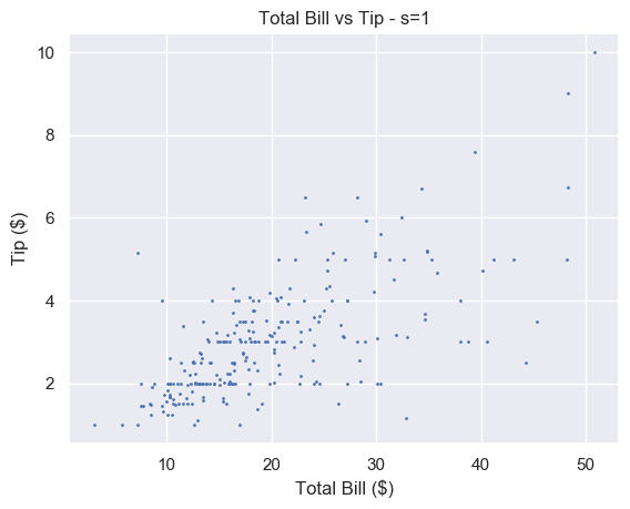
# Small s
plt.scatter(total_bill, tip, s=1)
plt.show()

A small number makes each marker small. Setting s=1 is too small for this plot and makes it hard to read. For some plots with a lot of data, setting s to a very small number makes it much easier to read. 

# Big s
plt.scatter(total_bill, tip, s=100)
plt.show()

Alternatively, a large number makes the markers bigger. This is too big for our plot and obscures a lot of the data.

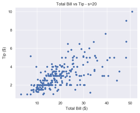
We think that s=20 strikes a nice balance for this particular plot.

# Just right
plt.scatter(total_bill, tip, s=20)
plt.show()

There is still some overlap between points but it is easier to spot. And unlike for s=1, you don’t have to strain to see the different markers. 

Matplotlib Scatter Marker Size – Array

If we pass an array to s, we set the size of each point individually. This is incredibly useful let’s use show more data on our scatter plot. We can use it to modify the size of our markers based on another variable. 

You also recorded the size of each of table you waited. This is stored in the NumPy array size_of_table. It contains integers in the range 1-6, representing the number of people you served.

# Select column 'size' and turn into a numpy array
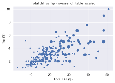
size_of_table = tips_df['size'].to_numpy() # Increase marker size to make plot easier to read
size_of_table_scaled = [3*s**2 for s in size_of_table] plt.scatter(total_bill, tip, s=size_of_table_scaled)
plt.show()

Not only does the tip increase when total bill increases, but serving more people leads to a bigger tip as well. This is in line with what we’d expect and it’s great our data fits our assumptions.

Why did we scale the size_of_table values before passing it to s? Because the change in size isn’t visible if we set s=1, …, s=6 as shown below.

So we first square each value and multiply it by 3 to make the size difference more pronounced. 

We should label everything on our graphs, so let’s add a legend.

Matplotlib Scatter Legend

To add a legend we use the plt.legend() function. This is easy to use with line plots. If we draw multiple lines on one graph, we label them individually using the label keyword. Then, when we call plt.legend(), matplotlib draws a legend with an entry for each line. 

But we have a problem. We’ve only got one set of data here. We cannot label the points individually using the label keyword.

How do we solve this problem?

We could create 6 different datasets, plot them on top of each other and give each a different size and label. But this is time-consuming and not scalable.

Fortunately, matplotlib has a scatter plot method we can use. It’s called the legend_elements() method because we want to label the different elements in our scatter plot. 

The elements in this scatter plot are different sizes. We have 6 different sized points to represent the 6 different sized tables. So we want legend_elements() to split our plot into 6 sections that we can label on our legend.

Let’s figure out how legend_elements() works. First, what happens when we call it without any arguments?

# legend_elements() is a method so we must name our scatter plot
scatter = plt.scatter(total_bill, tip, s=size_of_table_scaled) legend = scatter.legend_elements() print(legend)
# ([], [])

Calling legend_elements() without any parameters, returns a tuple of length 2. It contains two empty lists.

The docs tell us legend_elements() returns the tuple (handles, labels). Handles are the parts of the plot you want to label. Labels are the names that will appear in the legend. For our plot, the handles are the different sized markers and the labels are the numbers 1-6.  The plt.legend() function accepts 2 arguments: handles and labels. 

The plt.legend() function accepts two arguments: plt.legend(handles, labels). As scatter.legend_elements() is a tuple of length 2, we have two options. We can either use the asterisk * operator to unpack it or we can unpack it ourselves.

# Method 1 - unpack tuple using *
legend = scatter.legend_elements()
plt.legend(*legend) # Method 2 - unpack tuple into 2 variables
handles, labels = scatter.legend_elements()
plt.legend(handles, labels)

Both produce the same result. The matplotlib docs use method 1. Yet method 2 gives us more flexibility. If we don’t like the labels matplotlib creates, we can overwrite them ourselves (as we will see in a moment). 

Currently, handles and labels are empty lists. Let’s change this by passing some arguments to legend_elements().

There are 4 optional arguments but let’s focus on the most important one: prop.

Prop – the property of the scatter graph you want to highlight in your legend. Default is 'colors', the other option is 'sizes'.

We will look at different colored scatter plots in the next section. As our plot contains 6 different sized markers, we set prop='sizes'.

scatter = plt.scatter(total_bill, tip, s=size_of_table_scaled) handles, labels = scatter.legend_elements(prop='sizes')

Now let’s look at the contents of handles and labels.

>>> type(handles)
list
>>> len(handles)
6 >>> handles
[<matplotlib.lines.Line2D object at 0x1a2336c650>,
<matplotlib.lines.Line2D object at 0x1a2336bd90>,
<matplotlib.lines.Line2D object at 0x1a2336cbd0>,
<matplotlib.lines.Line2D object at 0x1a2336cc90>,
<matplotlib.lines.Line2D object at 0x1a2336ce50>,
<matplotlib.lines.Line2D object at 0x1a230e1150>]

Handles is a list of length 6. Each element in the list is a matplotlib.lines.Line2D object. You don’t need to understand exactly what that is. Just know that if you pass these objects to plt.legend(), matplotlib renders an appropriate 'picture'. For colored lines, it’s a short line of that color. In this case, it’s a single point and each of the 6 points will be a different size. 

It is possible to create custom handles but this is out of the scope of this article. Now let’s look at labels.

>>> type(labels)
list
>>> len(labels)
6 >>> labels
['$\\mathdefault{3}$', '$\\mathdefault{12}$', '$\\mathdefault{27}$', '$\\mathdefault{48}$', '$\\mathdefault{75}$', '$\\mathdefault{108}$']

Again, we have a list of length 6. Each element is a string. Each string is written using LaTeX notation '$...$'. So the labels are the numbers 3, 12, 27, 48, 75 and 108. 

Why these numbers? Because they are the unique values in the list size_of_table_scaled. This list defines the marker size. 

>>> np.unique(size_of_table_scaled)
array([ 3, 12, 27, 48, 75, 108])

We used these numbers because using 1-6 is not enough of a size difference for humans to notice. 

However, for our legend, we want to use the numbers 1-6 as this is the actual table size. So let’s overwrite labels. 

labels = ['1', '2', '3', '4', '5', '6']

Note that each element must be a string.

We now have everything we need to create a legend. Let’s put this together. 

# Increase marker size to make plot easier to read
size_of_table_scaled = [3*s**2 for s in size_of_table] # Scatter plot with marker sizes proportional to table size
scatter = plt.scatter(total_bill, tip, s=size_of_table_scaled) # Generate handles and labels using legend_elements method
handles, labels = scatter.legend_elements(prop='sizes') # Overwrite labels with the numbers 1-6 as strings
labels = ['1', '2', '3', '4', '5', '6'] # Add a title to legend with title keyword
plt.legend(handles, labels, title='Table Size')
plt.show()

Perfect, we have a legend that shows the reader exactly what the graph represents. It is easy to understand and adds a lot of value to the plot.

Now let’s look at another way to represent multiple variables on our scatter plot: color.

Matplotlib Scatter Plot Color

Color is an incredibly important part of plotting. It could be an entire article in itself. Check out the Seaborn docs for a great overview. 

Color can make or break your plot. Some color schemes make it ridiculously easy to understand the data. Others make it impossible. 

However, one reason to change the color is purely for aesthetics. 

We choose the color of points in plt.scatter() with the keyword c or color. 

You can set any color you want using an RGB or RGBA tuple (red, green, blue, alpha). Each element of these tuples is a float in [0.0, 1.0]. You can also pass a hex RGB or RGBA string such as '#1f1f1f'. However, most of the time you’ll use one of the 50+ built-in named colors. The most common are:

• 'b' or 'blue'
• 'r' or 'red'
• 'g' or 'green'
• 'k' or 'black'
• 'w' or 'white'

Here’s the plot of total_bill vs tip using different colors

For each plot, call plt.scatter() with total_bill and tip and set color (or c) to your choice

# Blue (the default value)
plt.scatter(total_bill, tip, color='b') # Red
plt.scatter(total_bill, tip, color='r') # Green
plt.scatter(total_bill, tip, c='g') # Black
plt.scatter(total_bill, tip, c='k')

Note: we put the plots on one figure to save space. We’ll cover how to do this in another article (hint: use plt.subplots())

Matplotlib Scatter Plot Different Colors

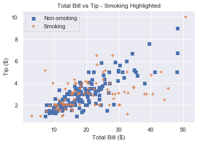
Our restaurant has a smoking area. We want to see if a group sitting in the smoking area affects the amount they tip.

We could show this by changing the size of the markers like above. But it doesn’t make much sense to do so. A bigger group logically implies a bigger marker. But marker size and being a smoker don’t have any connection and may be confusing for the reader. 

Instead, we will color our markers differently to represent smokers and non-smokers. 

We have split our data into four NumPy arrays: 

• x-axis – non_smoking_total_bill, smoking_total_bill
• y-axis – non_smoking_tip, smoking_tip

If you draw multiple scatter plots at once, matplotlib colors them differently. This makes it easy to recognize the different datasets.

plt.scatter(non_smoking_total_bill, non_smoking_tip)
plt.scatter(smoking_total_bill, smoking_tip)
plt.show()

This looks great. It’s very easy to tell the orange and blue markers apart. The only problem is that we don’t know which is which. Let’s add a legend. 

As we have 2 plt.scatter() calls, we can label each one and then call plt.legend().

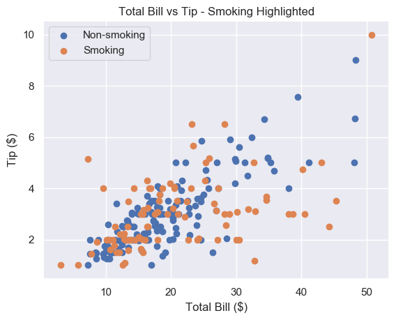
# Add label names to each scatter plot
plt.scatter(non_smoking_total_bill, non_smoking_tip, label='Non-smoking')
plt.scatter(smoking_total_bill, smoking_tip, label='Smoking') # Put legend in upper left corner of the plot
plt.legend(loc='upper left')
plt.show()

Much better. It seems that the smoker’s data is more spread out and flat than non-smoking data. This implies that smokers tip about the same regardless of their bill size. Let’s try to serve less smoking tables and more non-smoking ones.

This method works fine if we have separate data. But most of the time we don’t and separating it can be tedious. 

Thankfully, like with size, we can pass c an array/sequence.

Let’s say we have a list smoker that contains 1 if the table smoked and 0 if they didn’t.

plt.scatter(total_bill, tip, c=smoker)
plt.show()

Note: if we pass an array/sequence, we must the keyword c instead of color. Python raises a ValueError if you use the latter.

ValueError: 'color' kwarg must be an mpl color spec or sequence of color specs.
For a sequence of values to be color-mapped, use the 'c' argument instead.

Great, now we have a plot with two different colors in 2 lines of code. But the colors are hard to see. 

Matplotlib Scatter Colormap

A colormap is a range of colors matplotlib uses to shade your plots. We set a colormap with the cmap argument. All possible colormaps are listed here. 

We’ll choose 'bwr' which stands for blue-white-red. For two datasets, it chooses just blue and red.

If color theory interests you, we highly recommend this paper. In it, the author creates bwr. Then he argues it should be the default color scheme for all scientific visualizations. 

plt.scatter(total_bill, tip, c=smoker, cmap='bwr')
plt.show()

Much better. Now let’s add a legend.

As we have one plt.scatter() call, we must use scatter.legend_elements() like we did earlier. This time, we’ll set prop='colors'. But since this is the default setting, we call legend_elements() without any arguments. 

# legend_elements() is a method so we must name our scatter plot
scatter = plt.scatter(total_bill, tip, c=smoker_num, cmap='bwr') # No arguments necessary, default is prop='colors'
handles, labels = scatter.legend_elements() # Print out labels to see which appears first
print(labels)
# ['$\\mathdefault{0}$', '$\\mathdefault{1}$']

We unpack our legend into handles and labels like before. Then we print labels to see the order matplotlib chose. It uses an ascending ordering. So 0 (non-smokers) is first. 

Now we overwrite labels with descriptive strings and pass everything to plt.legend().

# Re-name labels to something easier to understand
labels = ['Non-Smokers', 'Smokers'] plt.legend(handles, labels)
plt.show()

This is a great scatter plot. It’s easy to distinguish between the colors and the legend tells us what they mean. As smoking is unhealthy, it’s also nice that this is represented by red as it suggests 'danger'. 

What if we wanted to swap the colors? 

Do the same as above but make the smoker list 0 for smokers and 1 for non-smokers. 

smokers_swapped = [1 - x for x in smokers]

Finally, as 0 comes first, we overwrite labels in the opposite order to before.

labels = ['Smokers', 'Non-Smokers']

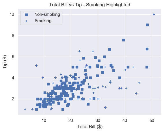
Matplotlib Scatter Marker Types

Instead of using color to represent smokers and non-smokers, we could use different marker types.

There are over 30 built-in markers to choose from. Plus you can use any LaTeX expressions and even define your own shapes. We’ll cover the most common built-in types you’ll see. Thankfully, the syntax for choosing them is intuitive. 

In our plt.scatter() call, use the marker keyword argument to set the marker type. Usually, the shape of the string reflects the shape of the marker. Or the string is a single letter matching to the first letter of the shape. 

Here are the most common examples:

• 'o' – circle (default)
• 'v' – triangle down
• '^' – triangle up
• 's' – square
• '+' – plus
• 'D' – diamond
• 'd' – thin diamond
• '$...$' – LaTeX syntax e.g. '$\pi$' makes each marker the Greek letter π. 

Let’s see some examples

For each plot, call plt.scatter() with total_bill and tip and set marker to your choice

# Circle
plt.scatter(total_bill, tip, marker='o') # Plus
plt.scatter(total_bill, tip, marker='+') # Diamond
plt.scatter(total_bill, tip, marker='D') # Triangle Up
plt.scatter(total_bill, tip, marker='^')

At the time of writing, you cannot pass an array to marker like you can with color or size. There is an open GitHub issue requesting that this feature is added. But for now, to plot two datasets with different markers, you need to do it manually.

# Square marker
plt.scatter(non_smoking_total_bill, non_smoking_tip, marker='s', label='Non-smoking') # Plus marker
plt.scatter(smoking_total_bill, smoking_tip, marker='+', label='Smoking') plt.legend(loc='upper left')
plt.show()

Remember that if you draw multiple scatter plots at once, matplotlib colors them differently. This makes it easy to recognise the different datasets. So there is little value in also changing the marker type. 

To get a plot in one color with different marker types, set the same color for each plot and change each marker. 

# Square marker, blue color
plt.scatter(non_smoking_total_bill, non_smoking_tip, marker='s', c='b' label='Non-smoking') # Plus marker, blue color
plt.scatter(smoking_total_bill, smoking_tip, marker='+', c='b' label='Smoking') plt.legend(loc='upper left')
plt.show()

Most would agree that different colors are easier to distinguish than different markers. But now you have the ability to choose.

Summary

You now know the 4 most important things to make excellent scatter plots. 

You can make basic matplotlib scatter plots. You can change the marker size to make the data easier to understand. And you can change the marker size based on another variable. 

You’ve learned how to choose any color imaginable for your plot. Plus you can change the color based on another variable. 

To add personality to your plots, you can use a custom marker type.

Finally, you can do all of this with an accompanying legend (something most Pythonistas don’t know how to use!). 

Where To Go From Here

Do you want to earn more money? Are you in a dead-end 9-5 job? Do you dream of breaking free and coding full-time but aren’t sure how to get started? 

Becoming a full-time coder is scary. There is so much coding info out there that it’s overwhelming. 

Most tutorials teach you Python and tell you to get a full-time job. 

That’s ok but why would you want another office job?

Don’t you crave freedom? Don’t you want to travel the world? Don’t you want to spend more time with your friends and family?

There are hardly any tutorials that teach you Python and how to be your own boss. And there are none that teach you how to make six figures a year.

Until now. 

We are full-time Python freelancers. We work from anywhere in the world. We set our own schedules and hourly rates. Our calendars are booked out months in advance and we have a constant flow of new clients. 

Sounds too good to be true, right?

Not at all. We want to show you the exact steps we used to get here. We want to give you a life of freedom. We want you to be a six-figure coder.

Click the link below to watch our pure-value webinar. We show you the exact steps to take you from where you are to a full-time Python freelancer. These are proven, no-BS methods that get you results fast.

https://tinyurl.com/python-freelancer-webinar

It doesn’t matter if you’re a Python novice or Python pro. If you are not making six figures/year with Python right now, you will learn something from this webinar.

Click the link below now and learn how to become a Python freelancer.

https://tinyurl.com/python-freelancer-webinar

References

• https://stackoverflow.com/questions/14827650/pyplot-scatter-plot-marker-size
• https://matplotlib.org/3.1.1/api/_as_gen/matplotlib.pyplot.scatter.html
• https://seaborn.pydata.org/generated/seaborn.scatterplot.html
• https://matplotlib.org/3.1.1/api/collections_api.html#matplotlib.collections.PathCollection.legend_elements
• https://blog.finxter.com/what-is-asterisk-in-python/
• https://matplotlib.org/3.1.1/api/markers_api.html#module-matplotlib.markers
• https://stackoverflow.com/questions/31726643/how-do-i-get-multiple-subplots-in-matplotlib
• https://matplotlib.org/3.1.0/gallery/color/named_colors.html
• https://matplotlib.org/3.1.0/tutorials/colors/colors.html#xkcd-colors
• https://github.com/matplotlib/matplotlib/issues/11155
• https://matplotlib.org/3.1.1/tutorials/colors/colormaps.html
• https://matplotlib.org/3.1.1/api/_as_gen/matplotlib.pyplot.legend.html
• https://matplotlib.org/tutorials/intermediate/legend_guide.html
• https://seaborn.pydata.org/tutorial/color_palettes.html
• https://cfwebprod.sandia.gov/cfdocs/CompResearch/docs/ColorMapsExpanded.pdf
• https://matplotlib.org/3.1.1/api/_as_gen/matplotlib.pyplot.subplots.html

The post Matplotlib Scatter Plot – Simple Illustrated Guide first appeared on Finxter.

Python comes with an extensive support of exceptions and exception handling. An exception event interrupts and, if uncaught, immediately terminates a running program. The most popular examples are the IndexError, ValueError, and TypeError.

An exception will immediately terminate your program. To avoid this, you can catch the exception with a try/except block around the code where you expect that a certain exception may occur. Here’s how you catch and print a given exception:

To catch and print an exception that occurred in a code snippet, wrap it in an indented try block, followed by the command "except Exception as e" that catches the exception and saves its error message in string variable e. You can now print the error message with "print(e)" or use it for further processing.

try: # ... YOUR CODE HERE ... #
except Exception as e: # ... PRINT THE ERROR MESSAGE ... # print(e)

Example 1: Catch and Print IndexError

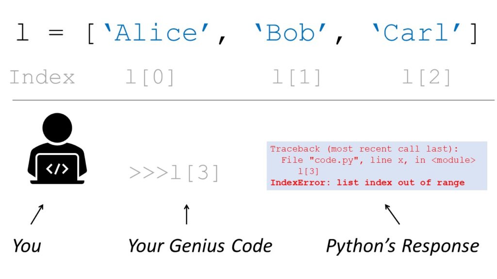
If you try to access the list element with index 100 but your lists consist only of three elements, Python will throw an IndexError telling you that the list index is out of range.

try: lst = ['Alice', 'Bob', 'Carl'] print(lst[3])
except Exception as e: print(e) print('Am I executed?')

Your genius code attempts to access the fourth element in your list with index 3—that doesn’t exist!

Fortunately, you wrapped the code in a try/catch block and printed the exception. The program is not terminated. Thus, it executes the final print() statement after the exception has been caught and handled. This is the output of the previous code snippet.

list index out of range
Am I executed?

Example 2: Catch and Print ValueError

The ValueError arises if you try to use wrong values in some functions. Here’s an example where the ValueError is raised because you tried to calculate the square root of a negative number:

import math try: a = math.sqrt(-2)
except Exception as e: print(e) print('Am I executed?')

The output shows that not only the error message but also the string 'Am I executed?' is printed.

math domain error
Am I executed?

Example 3: Catch and Print TypeError

Python throws the TypeError object is not subscriptable if you use indexing with the square bracket notation on an object that is not indexable. This is the case if the object doesn’t define the __getitem__() method. Here’s how you can catch the error and print it to your shell:

try: variable = None print(variable[0])
except Exception as e: print(e) print('Am I executed?')

The output shows that not only the error message but also the string 'Am I executed?' is printed.

'NoneType' object is not subscriptable
Am I executed?

I hope you’re now able to catch and print your error messages.

Summary

To catch and print an exception that occurred in a code snippet, wrap it in an indented try block, followed by the command "except Exception as e" that catches the exception and saves its error message in string variable e. You can now print the error message with "print(e)" or use it for further processing.

Where to Go From Here?

Enough theory, let’s get some practice!

To become successful in coding, you need to get out there and solve real problems for real people. That’s how you can become a six-figure earner easily. And that’s how you polish the skills you really need in practice. After all, what’s the use of learning theory that nobody ever needs?

Practice projects is how you sharpen your saw in coding!

Do you want to become a code master by focusing on practical code projects that actually earn you money and solve problems for people?

Then become a Python freelance developer! It’s the best way of approaching the task of improving your Python skills—even if you are a complete beginner.

Join my free webinar “How to Build Your High-Income Skill Python” and watch how I grew my coding business online and how you can, too—from the comfort of your own home.

Join the free webinar now!

The post How to Catch and Print Exception Messages in Python first appeared on Finxter.

The pandas.concat( ) function combines the data from multiple Series and/or DataFrames fast and in an intuitive manner. It is one of the most basic data wrangling operations used in Pandas. In general, we draw some conclusions from the data by analyzing it. The confidence in our conclusions increases as we include more variables or meta-data about our data. This is achieved by combining data from a variety of different data sources. The basic Pandas objects, Series, and DataFrames are created by keeping these relational operations in mind. For example, pd.concat([df1, df2]) concatenates two DataFrames df1, df2 together horizontally and results in a new DataFrame.

Pandas Concat Two or More DataFrames

The most important and widely used use-case of Pandas concat – pd.concat( ) is to concatenate DataFrames.

For example, when you’re buying a new smartphone, often you might like to compare the specifications and price of the phones. This makes you take an informed decision. Such a comparison can be viewed below as an example from the amazon website for recent OnePlus phones.

In the above image, the data about four different smartphones are concatenated with their features as an index.

Let us construct two DataFrames and combine them to see how it works.

>>> import pandas as pd
>>> df1 = pd.DataFrame(
... {"Key": ["A", "B", "A", "C"], "C1":[1, 2, 3, 4], "C2": [10, 20, 30, 40]})
>>> df1.index = ["L1", "L2", "L3", "L4"]
>>> print(df1) Key C1 C2
L1 A 1 10
L2 B 2 20
L3 A 3 30
L4 C 4 40
>>> df2 = pd.DataFrame(
... {"Key": ["A", "B", "C", "D"], "C3": [100, 200, 300, 400]})
>>> df2.index = ["R1", "R2", "R3", "R4"]
>>> print(df2) Key C3
R1 A 100
R2 B 200
R3 C 300
R4 D 400

From the official Pandas documentation of Pandas concat;

The two major arguments used in pandas.concat( ) from the above image are,

• objs – A sequence of Series and/or DataFrame objects
• axis – Axis along which objs are concatenated

Out of the two arguments, objs remains constant. But, based on the value of the axis, the concatenation operation differs. Possible values of the axis are,

• axis = 0 – Concatenate or stack the DataFrames down the rows
• axis = 1 – Concatenate or stack the DataFrames along the columns

Remember this axis argument functionality, because it comes in many other Pandas functions. Let us see them in action using the above created Dataframes.

1. Row-Wise Concatenation (axis = 0 / ’index’)

>>> df3 = pd.concat([df1, df2], axis=0)
>>> print(df3) Key C1 C2 C3
L1 A 1.0 10.0 NaN
L2 B 2.0 20.0 NaN
L3 A 3.0 30.0 NaN
L4 C 4.0 40.0 NaN
R1 A NaN NaN 100.0
R2 B NaN NaN 200.0
R3 C NaN NaN 300.0
R4 D NaN NaN 400.0
>>> df3_dash = pd.concat([df1, df2])
>>> print(df3_dash) Key C1 C2 C3
L1 A 1.0 10.0 NaN
L2 B 2.0 20.0 NaN
L3 A 3.0 30.0 NaN
L4 C 4.0 40.0 NaN
R1 A NaN NaN 100.0
R2 B NaN NaN 200.0
R3 C NaN NaN 300.0
R4 D NaN NaN 400.0
>>> print(len(df3) == len(df1) + len(df2))
True

Any number of DataFrames can be given in the first argument which has a list of DataFrames like [df1, df2, df3, ..., dfn].

Some observations from the above results:

• Note the outputs of df3 and df3_dash are the same. So, we need not explicitly mention the axis when we want to concatenate down the rows.
• The number of rows in the output DataFrame = Total number of rows in all the input DataFrames.
• The columns of the output DataFrame = Combination of distinct columns of all the input DataFrames.
• There are unique columns present in the input DataFrames. The corresponding values at the row labels of different input DataFrames are filled with NaNs (Not a Number – missing values) in the output DataFrame.

Let’s visualize the above process in the following animation:

2. Column-Wise Concatenation (axis = 1 / ’columns’)

>>> df3 = pd.concat([df1, df2], axis=1)
>>> print(df3) Key C1 C2 Key C3
L1 A 1.0 10.0 NaN NaN
L2 B 2.0 20.0 NaN NaN
L3 A 3.0 30.0 NaN NaN
L4 C 4.0 40.0 NaN NaN
R1 NaN NaN NaN A 100.0
R2 NaN NaN NaN B 200.0
R3 NaN NaN NaN C 300.0
R4 NaN NaN NaN D 400.0
>>> print("The unique row indexes of df1 and df2:", '\n\t', df1.index.append(df2.index).unique())
The unique row indexes of df1 and df2: Index(['L1', 'L2', 'L3', 'L4', 'R1', 'R2', 'R3', 'R4'], dtype='object')
>>> print("The row indexes of df3:", "\n\t", df3.index)
The row indexes of df3: Index(['L1', 'L2', 'L3', 'L4', 'R1', 'R2', 'R3', 'R4'], dtype='object')
>>> print("The column indexes of df1 and df2:", "\n\t", df1.columns.append(df2.columns))
The column indexes of df1 and df2: Index(['Key', 'C1', 'C2', 'Key', 'C3'], dtype='object')
>>> print("The column indexes of df3:", "\n\t", df3.columns)
The column indexes of df3: Index(['Key', 'C1', 'C2', 'Key', 'C3'], dtype='object')

Some observations from the above results:

• The DataFrames are concatenated side by side.
• The columns in the output DataFrame = Total columns in all the input DataFrames.
• Rows in the output DataFrame = Unique rows in all the input DataFrames.
• There are unique rows present in all the input DataFrames. The corresponding values at the column labels of different input DataFrames are filled with NaNs (Not a Number – missing values) in the output DataFrame.

Let’s visualize the above process in the following animation:

Pandas Concat Columns

Please take a look at the initial OnePlus phones comparison table from the amazon website. A column in that table constitutes all the specifications of a given smartphone. Such all equivalent specifications (row labels) of all varieties (phones – column labels) are concatenated as columns to form the final comparison table.

So, to concatenate columns, we should have the same row indexes. In Pandas, the Series data structure is exactly designed to represent the columns and their combination forms the DataFrame data structure.

Let us construct two Series and concatenate them as columns to form a resultant DataFrame.

>>> ser1 = pd.Series([10, 20, 30, 40], name='C1')
>>> ser2 = pd.Series([100, 200, 300, 400], name='C2')
>>> print("Series 1:", "\n", ser1, "\n\n", "Series 2:", "\n", ser2)
Series 1:
0 10
1 20
2 30
3 40
Name: C1, dtype: int64 Series 2:
0 100
1 200
2 300
3 400
Name: C2, dtype: int64
>>> df = pd.concat([ser1, ser2], axis=1)
>>> print("DataFrame:", "\n", df)
DataFrame: C1 C2
0 10 100
1 20 200
2 30 300
3 40 400

Pandas Concat MultiIndex

Let us consider a use-case where we have hourly weather data for 4 hours about two cities. The data that we have are only the temperature (degC) and wind speed (kmph). One way of storing their data is to store them in different DataFrames per city. It can be done the following way,

>>> Date_Hourly = pd.date_range(start = '2020-11-20', periods = 4, freq = 'H')
>>> df_city1 = pd.DataFrame(
... {"temp(degC)": [27, 24, 22, 20],
... "windspeed(kmph)": [18, 17, 17, 18]},
... index = Date_Hourly
... )
>>> df_city2 = pd.DataFrame(
... {"temp(degC)": [30, 33, 33, 34],
... "windspeed(kmph)": [23, 25, 27, 30]},
... index = Date_Hourly
... )
>>> print("Weather Data of City 1:", "\n", df_city1)
Weather Data of City 1: temp(degC) windspeed(kmph)
2020-11-20 00:00:00 27 18
2020-11-20 01:00:00 24 17
2020-11-20 02:00:00 22 17
2020-11-20 03:00:00 20 18
>>> print("Weather Data of City 2:", "\n", df_city2)
Weather Data of City 2: temp(degC) windspeed(kmph)
2020-11-20 00:00:00 30 23
2020-11-20 01:00:00 33 25
2020-11-20 02:00:00 33 27
2020-11-20 03:00:00 34 30

Now, we might want to collect data of two cities into one DataFrame for easier analysis. MultiIndex keys serve as identifiers to specify the source of the data. This can be achieved by MultiIndex concatenation.

Multi-Index Concatenation is done in two ways;

1. Row-Wise Concatenation (axis = 0 / ’index’)

>>> df_concat_rowwise = pd.concat([df_city1, df_city2], axis=0, keys=['City1', 'City2'])
>>> print("Row-Wise Multi-Index Concatenation:", "\n", df_concat_rowwise)
Row-Wise Multi-Index Concatenation: temp(degC) windspeed(kmph)
City1 2020-11-20 00:00:00 27 18 2020-11-20 01:00:00 24 17 2020-11-20 02:00:00 22 17 2020-11-20 03:00:00 20 18
City2 2020-11-20 00:00:00 30 23 2020-11-20 01:00:00 33 25 2020-11-20 02:00:00 33 27 2020-11-20 03:00:00 34 30

2. Column-Wise Concatenation (axis = 1 / ’columns’)

>>> df_concat_rowwise = pd.concat([df_city1, df_city2], axis=1, keys=['City1', 'City2']) >>> print("Column-Wise Multi-Index Concatenation:", "\n", df_concat_colwise)
Column-Wise Multi-Index Concatenation: City1 City2 temp(degC) windspeed(kmph) temp(degC) windspeed(kmph)
2020-11-20 00:00:00 27 18 30 23
2020-11-20 01:00:00 24 17 33 25
2020-11-20 02:00:00 22 17 33 27
2020-11-20 03:00:00 20 18 34 30

The same can be achieved for many cities. After concatenation, all of the data is in one single DataFrame. This makes us analyze the weather efficiently instead of fetching data from multiple sources.

Pandas concat vs append

Concatenation along the rows (axis = 0) is very common. If you observe the weather data scenario after each hour data gets appended in the next row. So, for that purpose, a method called append( ) is built on top of DataFrame to append another DataFrame row-wise. This makes you achieve the same results as pd.concat( ) with few keystrokes.

It can be implemented as follows,

>>> df1 = pd.DataFrame({'C1': ['A', 'B', 'C', 'D']})
>>> df2 = pd.DataFrame({'C1': ['E', 'F', 'G', 'H']})
>>> print("DataFrame 1:", "\n", df1)
DataFrame 1: C1
0 A
1 B
2 C
3 D
>>> print("DataFrame 2:", "\n", df2)
DataFrame 2: C1
0 E
1 F
2 G
3 H
>>> pd.concat([df1, df2]) C1
0 A
1 B
2 C
3 D
0 E
1 F
2 G
3 H
>>> df1.append(df2) C1
0 A
1 B
2 C
3 D
0 E
1 F
2 G
3 H

You can observe above the same results for pd.concat([df1, df2]) and df1.append(df2).

Pandas concat slow

Each and every time we do a concatenation operation, it creates a new DataFrame. DataFrame concatenation operates equivalent to an SQL join operation. So, the output DataFrame’s index is formed first by join operation. Resolving all the mismatches between indexes of input DataFrames makes it slow. In some scenarios, indexes might not be of importance. In such cases, we can ignore indexes to make the concat operation faster.

Ignoring the index is done by the following way,

>>> df = pd.DataFrame({'C1': [10, 20, 30, 40]}, index=['R1', 'R2', 'R3', 'R4'])
>>> df C1
R1 10
R2 20
R3 30
R4 40
>>> df.reset_index(drop=True) C1
0 10
1 20
2 30
3 40

Along with concat, all other Pandas functions are executed by utilizing only a single core in the CPU. Operations on smaller datasets run in a seamless manner. As the dataset size increases, the functions of Pandas start to throttle because they do only one operation at once.

Modin is the python package created to speed up the execution of Pandas functions. It distributes the computation load to all the available cores. It does so by fragmenting the DatFrame and making the function run on DataFrame fragments in other cores parallelly. Please look after this article to know about it in detail.

The post How Does Pandas Concat Work? first appeared on Finxter.

The next(iterator) function is one of Python’s built-in functions—so, you can use it without importing any library. It returns the next value from the iterator you pass as a required first argument. An optional second argument default returns the passed default value in case the iterator doesn’t provide a next value.

Syntax:

next(iterator, <default>)

---

Arguments:

• iterator – the next element is retrieved from the iterator
• default (optional) – return value if iterator is exhausted (it doesn’t have a next element)

Related Tutorials:

• Python Keywords Cheat Sheet
• Python Iterators
• Yield Keyword
• Python Lists

Example 1: No Default Value

The following example shows the next() function in action—without using a default value in case the iterator is empty.

users = ['Alice', 'Bob', 'Carl', 'David'] # convert the list to an iterator
users_iterator = iter(users) x = next(users_iterator)
print(x)
# Output: 'Alice' x = next(users_iterator)
print(x)
# Output: 'Bob' x = next(users_iterator)
print(x)
# Output: 'Carl' x = next(users_iterator)
print(x)
# Output: 'David'

Each time you call next(iterator), the iterator returns the next element in the iterator over the Python list users.

But what happens if you call the next() function once more on the now empty users_iterator object?

x = next(users_iterator)
print(x) '''
Traceback (most recent call last): File "C:\Users\xcent\Desktop\Finxter\Blog\HowToConvertBooleanToStringPython\code.py", line 22, in <module> x = next(users_iterator)
StopIteration '''

Python throws a StopIteration error.

Let’s learn how to fix this!

Example 2: With Default Value

Not providing Python a solution to the problem that the iterator may be empty is a common source of errors! You can fix the errors by passing the optional default argument:

x = next(users_iterator, 42)
print(x)
# 42

Now, you cannot crash the next(...) function anymore! Go ahead and try it…

Interactive Shell

The interactive code shell offers you a way to try your newly gained skill—understanding the next() function. Can you crash the script by changing the default value?

Exercise: Run the code in the interactive shell. Now, change the default value & run again!

Where to Go From Here?

Enough theory, let’s get some practice!

To become successful in coding, you need to get out there and solve real problems for real people. That’s how you can become a six-figure earner easily. And that’s how you polish the skills you really need in practice. After all, what’s the use of learning theory that nobody ever needs?

Practice projects is how you sharpen your saw in coding!

Do you want to become a code master by focusing on practical code projects that actually earn you money and solve problems for people?

Then become a Python freelance developer! It’s the best way of approaching the task of improving your Python skills—even if you are a complete beginner.

Join my free webinar “How to Build Your High-Income Skill Python” and watch how I grew my coding business online and how you can, too—from the comfort of your own home.

Join the free webinar now!

The post Python next() first appeared on Finxter.

You may encounter a special ValueError when working with Python’s math module.

ValueError: math domain error

Python raises this error when you try to do something that is not mathematically possible or mathematically defined.

To understand this error, have a look at the definition of the domain:

“The domain of a function is the complete set of possible values of the independent variable. Roughly speaking, the domain is the set of all possible (input) x-values which result in a valid (output) y-value.” (source)

The domain of a function is the set of all possible input values. If Python throws the ValueError: math domain error, you’ve passed an undefined input into the math function. Fix the error by passing a valid input for which the function is able to calculate a numerical output.

Here are a few examples:

Python Math Domain Error Sqrt

The math domain error appears if you pass a negative argument into the math.sqrt() function. It’s mathematically impossible to calculate the square root of a negative number without using complex numbers. Python doesn’t get that and throws a ValueError: math domain error.

Here’s a minimal example:

from math import sqrt
print(sqrt(-1)) '''
Traceback (most recent call last): File "C:\Users\xcent\Desktop\Finxter\Blog\code.py", line 2, in <module> print(sqrt(-1))
ValueError: math domain error '''

You can fix the math domain error by using the cmath package that allows the creation of complex numbers:

from cmath import sqrt
print(sqrt(-1))
# 1j

Python Math Domain Error Log

The math domain error for the math.log() function appears if you pass a zero value into it—the logarithm is not defined for value 0.

Here’s the code on an input value outside the domain of the logarithm function:

from math import log
print(log(0))

The output is the math domain error:

Traceback (most recent call last): File "C:\Users\xcent\Desktop\Finxter\Blog\code.py", line 3, in <module> print(log(0))
ValueError: math domain error

You can fix this error by passing a valid input value into the math.log() function:

from math import log
print(log(0.000001))
# -13.815510557964274

This error can sometimes appear if you pass a very small number into it—Python’s float type cannot express all numbers. To pass a value “close to 0”, use the Decimal module with higher precision, or pass a very small input argument such as:

math.log(sys.float_info.min)

Python Math Domain Error Acos

The math domain error for the math.acos() function appears if you pass a value into it for which it is not defined—arccos is only defined for values between -1 and 1.

Here’s the wrong code:

import math
print(math.acos(2))

The output is the math domain error:

Traceback (most recent call last): File "C:\Users\xcent\Desktop\Finxter\Blog\code.py", line 3, in <module> print(math.acos(2))
ValueError: math domain error

You can fix this error by passing a valid input value between [-1,1] into the math.acos() function:

import math
print(math.acos(0.5))
# 1.0471975511965979

Python Math Domain Error Asin

The math domain error for the math.asin() function appears if you pass a value into it for which it is not defined—arcsin is only defined for values between -1 and 1.

Here’s the erroneous code:

import math
print(math.asin(2))

The output is the math domain error:

Traceback (most recent call last): File "C:\Users\xcent\Desktop\Finxter\Blog\code.py", line 3, in <module> print(math.asin(2))
ValueError: math domain error

You can fix this error by passing a valid input value between [-1,1] into the math.asin() function:

import math
print(math.asin(0.5))
# 0.5235987755982989

Python Math Domain Error Pow

The math domain error for the math.pow(a,b) function to calculate a**b appears if you pass a negative base value into it and try to calculate a negative power of it. The reason it is not defined is that any negative number to the power of 0.5 would be the square number—and thus, a complex number. But complex numbers are not defined by default in Python!

import math
print(math.pow(-2, 0.5))

The output is the math domain error:

Traceback (most recent call last): File "C:\Users\xcent\Desktop\Finxter\Blog\code.py", line 3, in <module> print(math.pow(-2, 0.5))
ValueError: math domain error

If you need a complex number, a^b must be rewritten into e^{b ln a}. For example:

import cmath
print(cmath.exp(0.5 * cmath.log(-2)))
# (8.659560562354932e-17+1.414213562373095j)

You see, it’s a complex number!

NumPy Math Domain Error — np.log(x)

import numpy as np
import matplotlib.pyplot as plt # Plotting y = log(x)
fig, ax = plt.subplots()
ax.set(xlim=(-5, 20), ylim=(-4, 4), title='log(x)', ylabel='y', xlabel='x')
x = np.linspace(-10, 20, num=1000)
y = np.log(x) plt.plot(x, y)

This is the graph of log(x). Don’t worry if you don’t understand the code, what’s more important is the following point. You can see that log(x) tends to negative infinity as x tends to 0. Thus, it is mathematically meaningless to calculate the log of a negative number. If you try to do so, Python raises a math domain error.

>>> math.log(-10)
Traceback (most recent call last): File "<stdin>", line 1, in <module>
ValueError: math domain error

Where to Go From Here?

Enough theory, let’s get some practice!

To become successful in coding, you need to get out there and solve real problems for real people. That’s how you can become a six-figure earner easily. And that’s how you polish the skills you really need in practice. After all, what’s the use of learning theory that nobody ever needs?

Practice projects is how you sharpen your saw in coding!

Do you want to become a code master by focusing on practical code projects that actually earn you money and solve problems for people?

Then become a Python freelance developer! It’s the best way of approaching the task of improving your Python skills—even if you are a complete beginner.

Join my free webinar “How to Build Your High-Income Skill Python” and watch how I grew my coding business online and how you can, too—from the comfort of your own home.

Join the free webinar now!

The post Python Math Domain Error (How to Fix This Stupid Bug) first appeared on Finxter.