Category: Python-Tut

The name agg is short for aggregate. To aggregate is to summarize many observations into a single value that represents a certain aspect of the observed data.

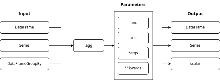
The .agg() function can process a dataframe, a series, or a grouped dataframe. It can execute many aggregation functions, e.g. ‘mean’, ‘max’,… in a single call along one of the axis. It can also execute lambda functions. Read on for examples.    

We will use a dataset of FIFA players. Find the dataset here.

Basic Setup using Jupyter Notebook

Let’s start by importing pandas and loading our dataset.

import pandas as pd
df_fifa_soccer_players = pd.read_csv('fifa_cleaned.csv')
df_fifa_soccer_players.head()

To increase readability, we will work with a subset of the data. Let’s create the subset by selecting the columns we want to have in our subset and create a new dataframe.

df_fifa_soccer_players_subset = df_fifa_soccer_players[['nationality', 'age', 'height_cm', 'weight_kgs', 'overall_rating', 'value_euro', 'wage_euro']]
df_fifa_soccer_players_subset.head()

Basic Aggregation

Pandas provides a variety of built-in aggregation functions. For example, pandas.DataFrame.describe. When applied to a dataset, it returns a summary of statistical values. 

df_fifa_soccer_players_subset.describe()

To understand aggregation and why it is helpful, let’s have a closer look at the data returned. 

Example: Our dataset contains records for 17954 players. The youngest player is 17 years of age and the oldest player is 46 years old. The mean age is 25 years. We learn that the tallest player is 205 cm tall and the average player’s height is around 175 cm. With a single line of code, we can answer a variety of statistical questions about our data. The describe function identifies numeric columns and performs the statistical aggregation for us. Describe also excluded the column nationality that contains string values.

To aggregate is to summarize many observations into a single value that represents a certain aspect of the observed data.

Pandas provides us with a variety of pre-built aggregate functions.

Functions	Description
mean()	returns the mean of a set of values
sum()	returns the sum of a set of values
count()	returns the count of a set of values
std()	returns the standard deviation of a set of values
min()	returns the smallest value of a set of values
max()	returns the largest value of a set of values
describe()	returns a collection of statistical values of a set of values
size()	returns the size of a set of values
first()	returns the first value of a set of values
last()	returns the last value of a set of values
nth()	returns the nth value of a set of values
sem()	returns the standard error of the mean of a set of value
var()	returns the variance of a set of values
nunique()	returns the count of unique values of a set of values

Let’s use another function from the list above. We can be more specific and request the ‘sum’ for the ‘value_euro’ series. This column contains the market value of a player. We select the column or series ‘value_euro’ and execute the pre-build sum() function.

df_fifa_soccer_players_subset['value_euro'].sum()
# 43880780000.0

Pandas returned us the requested value. Let’s get to know an even more powerful pandas method for aggregating data.

The ‘pandas.DataFrame.agg’ Method

Function Syntax

The .agg() function can take in many input types. The output type is, to a large extent, determined by the input type. We can pass in many parameters to the .agg() function. 

The “func” parameter:

• is by default set to None 
• contains one or many functions that aggregate the data
• supports pre-defined pandas aggregate functions
• supports lambda expressions
• supports the dataframe.apply() method for specific function calls

The “axis” parameter:

• is by default set to 0 and applies functions to each column
• if set to 1 applies functions to rows
• can hold values:
  • 0 or ‘index’
  • 1 or ‘columns’

What about *args and **kwargs:

• we use these placeholders, if we do not know in advance how many arguments we will need to pass into the function
• when arguments are of the same type, we use *args
• When arguments are of different types, we use **kwargs.

Agg method on a Series

Let’s see the .agg() function in action. We request some of the pre-build aggregation functions for the ‘wage_euro’ series. We use the function parameter and provide the aggregate functions ‌we want to execute as a list. And let’s save the resulting series in a variable. 

wage_stats = df_fifa_soccer_players_subset['wage_euro'].agg(['sum', 'min', 'mean', 'std', 'max'])
print(wage_stats)

Pandas uses scientific notation for large and small floating-point numbers. To convert the output to a familiar format, we must move the floating point to the right as shown by the plus sign. The number behind the plus sign represents the amount of steps.

Let’s do this together for some values.

The sum of all wages is 175,347,000€ (1.753470e+08)

The mean of the wages is 9902.135€ (9.902135e+03)

We executed many functions on a series input source. Thus our variable ‘wage_stats’ is of the type Series because. 

type(wage_stats)
# pandas.core.series.Series

See below how to extract, for example, the ‘min’ value from the variable and the data type returned.

wage_stats_min = wage_stats['min']
print(wage_stats_min)
# 1000.0 print(type(wage_stats_min))
# numpy.float64

The data type is now a scalar.

If we execute a single function on the same data source (series), the type returned is a scalar.

wage_stats_max = df_fifa_soccer_players_subset['wage_euro'].agg('max')
print(wage_stats_max)
# 565000.0 print(type(wage_stats_max))
# numpy.float64

Let’s use one more example to understand the relation between the input type and the output type.

We will use the function “nunique” which will give us the count of unique nationalities. Let’s apply the function in two code examples. We will reference the series ‘nationality’ both times. The only difference will be the way we pass the function “nunique” into our agg() function.

nationality_unique_series = df_fifa_soccer_players_subset['nationality'].agg({'nationality':'nunique'})
print(nationality_unique_series)
# nationality 160
# Name: nationality, dtype: int64 print(type(nationality_unique_series))
# pandas.core.series.Series

When we use a dictionary to pass in the “nunique” function, the output type is a series.

nationality_unique_int = df_fifa_soccer_players_subset['nationality'].agg('nunique')
print(nationality_unique_int)
# 160 print(type(nationality_unique_int))
# int

When we pass the “nunique” function directly into agg() the output type is an integer.

Agg method on a DataFrame

Passing the aggregation functions as a Python list

One column represents a series. We will now select two columns as our input and so work with a dataframe.

Let’s select the columns ‘height_cm’ and ‘weight_kgs’.

We will execute the functions min(), mean() and max(). To select a two-dimensional data (dataframe), we need to use double brackets. We will round the results to two decimal points.

Let’s store the result in a variable.

height_weight = df_fifa_soccer_players_subset[['height_cm', 'weight_kgs']].agg(['min', 'mean', 'max']).round(2)
print(height_weight)

We get a data frame containing rows and columns. Let’s confirm this observation by checking the type of the ‘height_weight’ variable.

print(type(height_weight))
# pandas.core.frame.DataFrame

We will now use our newly created dataframe named ‘height_weight’ to use the ‘axis’ parameter. The entire dataframe contains numeric values.

We define the functions and pass in the axis parameter. I used the count() and sum() functions to show the effect of the axis parameter. The resulting values make little sense. This is also the reason why I do not rename the headings to restore the lost column names.

height_weight.agg(['count', 'sum'], axis=1)

We aggregated along the rows. Returning the count of items and the sum of item values in each row.

Passing the aggregation functions as a python dictionary

Now let’s apply different functions to the individual sets in our dataframe. We select the sets ‘overall_rating’ and ‘value_euro’. We will apply the functions std(), sem() and mean() to the ‘overall_rating’ series, and the functions min() and max() to the ‘value_euro’ series.

rating_value_euro_dict = df_fifa_soccer_players_subset[['overall_rating', 'value_euro']].agg({'overall_rating':['std', 'sem', 'mean'], 'value_euro':['min', 'max']})
print(rating_value_euro_dict)

The dataframe contains calculated and empty (NaN) values. Let’s quickly confirm the type of our output.

print(type(rating_value_euro_dict))
# pandas.core.frame.DataFrame

Passing the aggregation functions as a Python tuple

We will now repeat the previous example.

We will use tuples instead of a dictionary to pass in the aggregation functions. Tuple have limitations. We can only pass one aggregation function within a tuple. We also have to name each tuple. 

rating_value_euro_tuple = df_fifa_soccer_players_subset[['overall_rating', 'value_euro']].agg(overall_r_std=('overall_rating', 'std'),overall_r_sem=('overall_rating', 'sem'),overall_r_mean=('overall_rating', 'mean'),value_e_min=('value_euro', 'min'),value_e_max=('value_euro', 'max'))
print(rating_value_euro_tuple)

Agg method on a grouped DataFrame

Grouping by a single column

The ‘groupby’ method creates a grouped dataframe. We will now select the columns ‘age’ and ‘wage_euro’ and group our dataframe using the column ‘age’. On our grouped dataframe we will apply the agg() function using the functions count(), min(), max() and mean().

age_group_wage_euro = df_fifa_soccer_players_subset[['age', 'wage_euro']].groupby('age').aggage(['count', 'min', 'max', 'mean'])
print(age_group_wage_euro)

Every row represents an age group. The count value shows how many players fall into the age group. The min, max and mean values aggregate the data of the age-group members.

Multiindex

One additional aspect of a grouped dataframe is the resulting hierarchical index. We also call it multiindex.

We can see that the individual columns of our grouped dataframe are at different levels. Another way to view the hierarchy is to request the columns for the particular dataset.

print(age_group_wage_euro.columns)

Working with a multiindex is a topic for another blog post. To use the tools that we have discussed, let’s flatten the multiindex and reset the index. We need the following functions:

• droplevel()
• reset_index()

age_group_wage_euro_flat = age_group_wage_euro.droplevel(axis=1, level=0).reset_index()
print(age_group_wage_euro_flat.head())

The resulting dataframe columns are now flat. We lost some information during the flattening process. Let’s rename the columns and return some of the lost context.

age_group_wage_euro_flat.columns = ['age', 'athlete_count', 'min_wage_euro', 'max_wage_euro', 'mean_wage_euro']
print(age_group_wage_euro_flat.head())

Grouping by multiple columns

Grouping by multiple columns creates even more granular subsections.

Let’s use ‘age’ as the first grouping parameter and ‘nationality’ as the second. We will aggregate the resulting group data using the columns ‘overall_rating’ and ‘height_cm’. We are by now familiar with the aggregation functions used in this example.

df_fifa_soccer_players_subset.groupby(['age', 'nationality']).agg({'overall_rating':['count', 'min', 'max', 'mean'], 'height_cm':['min', 'max', 'mean']})

Every age group contains nationality groups. The aggregated athletes data is within the nationality groups.

Custom aggregation functions

We can write and execute custom aggregation functions to answer very specific questions.

Let’s have a look at the inline lambda functions.

Lambda functions are so-called anonymous functions. They are called this way because they do not have a name. Within a lambda function, we can execute multiple expressions. We will go through several examples to see lambda functions in action.

In pandas lambda functions live inside the “DataFrame.apply()” and the “Series.appy()” methods. We will use the DataFrame.appy() method to execute functions along both axes. Let’s have a look at the basics first.

Function Syntax

The DataFrame.apply() function will execute a function along defined axes of a DataFrame. The functions that we will execute in our examples will work with Series objects passed into our custom functions by the apply() method. Depending on the axes that we will select, the Series will comprise out of a row or a column or our data frame.

The “func” parameter:

• contains a function applied to a column or a row of the data frame

The “axis” parameter:

• is by default set to 0 and will pass a series of column data
• if set to 1 will pass a series of the row data
• can hold values:
  • 0 or ‘index’
  • 1 or ‘columns’

The “raw” parameter:

• is a boolean value
•  is by default set to False
• can hold values:
  • False -> a Series object is passed to the function
  • True -> a ndarray object is passed to the function

The “result_type” parameter:

• can only apply when the axis is 1 or ‘columns’
• can hold values:
  • ‘expand’
  • ‘reduce’
  • ‘broadcast’

 The “args()” parameter:

• additional parameters for the function as tuple

The **kwargs parameter:

• additional parameters for the function as key-value pairs

Filters

Let’s have a look at filters. They will be very handy as we explore our data.

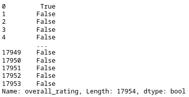
In this code example, we create a filter named filt_rating. We select our dataframe and the column overall_rating. The condition >= 90 returns True if the value in the overall_rating column is 90 or above.

Otherwise, the filter returns False.

filt_rating = df_fifa_soccer_players_subset['overall_rating'] >= 90
print(filt_rating)

The result is a Series object containing the index, and the correlated value of True or False.

Let’s apply the filter to our dataframe. We call the .loc method and pass in the filter’s name as a list item. The filter works like a mask. It covers all rows that have the value False. The remaining rows match our filter criteria of overall_rating >= 90.

df_fifa_soccer_players_subset.loc[filt_rating]

Lambda functions

Let’s recreate the same filter using a lambda function. We will call our filter filt_rating_lambda.

Let’s go over the code. We specify the name of our filter and call our dataframe. Pay attention to the double square brackets. We use them to pass a dataframe and not a Series object to the .appy() method.

Inside .apply() we use the keyword ‘lambda’ to show that we are about to define our anonymous function. The ‘x’ represents the Series passed into the lambda function.

The series contains the data from the overall_rating column. After the semicolumn, we use the placeholder x again. Now we apply a method called ge(). It represents the same condition we used in our first filter example “>=” (greater or equal).

We define the integer value 90 and close the brackets on our apply function. The result is a dataframe that contains an index and only one column of boolean values. To convert this dataframe to a Series we use the squeeze() method.

filt_rating_lambda = df_fifa_soccer_players_subset[['overall_rating']].apply(lambda x:x.ge(90)).squeeze()
print(filt_rating_lambda)

Let’s use our filter. Great, we get the same result as in our first filter example.

df_fifa_soccer_players_subset.loc[filt_rating_lambda]

We now want to know how many players our filter returned. Let’s first do it without a lambda function and then use a lambda function to see the same result. We are counting the lines or records.

df_fifa_soccer_players_subset.loc[filt_rating_lambda].count()

df_fifa_soccer_players_subset.apply(lambda x:x.loc[filt_rating_lambda]).count()

Great. Now let’s put us in a place where we actually need to use the apply() method and a lambda function. We want to use our filter on a grouped data-frame.

Let’s group by nationality to see the distribution of these amazing players. The output will contain all columns. This makes the code easier to read.

df_fifa_soccer_players_subset.groupby('nationality').loc[filt_rating_lambda]

Pandas tells us in this error message that we can not use the ‘loc’ method on a grouped dataframe object.

Let’s now see how we can solve this problem by using a lambda function. Instead of using the ‘loc’ function on the grouped dataframe we use the apply() function. Inside the apply() function we define our lambda function. Now we use the ‘loc’ method on the variable ‘x’ and pass our filter. 

df_fifa_soccer_players_subset.groupby('nationality').apply(lambda x:x.loc[filt_rating_lambda])

Axis parameter of the apply() function

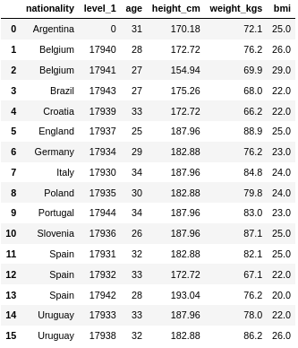
Now let’s use the axis parameter to calculate the Body-Mass-Index (BMI) for these players. Until now we have used the lambda functions on the columns of our data.

The ‘x’ variable was a representation of the individual column. We set the axis parameter to ‘1’. The ‘x’ variable in our lambda function will now represent the individual rows of our data.

Before we calculate the BMI let’s create a new dataframe and define some columns. We will call our new dataframe ‘df_bmi’. 

df_bmi = df_fifa_soccer_players_subset.groupby('nationality')[['age', 'height_cm', 'weight_kgs']].apply(lambda x:x.loc[filt_rating_lambda])
print(df_bmi)

Now let’s reset the index. 

df_bmi = df_bmi.reset_index()
print(df_bmi)

We calculate the BMI as follows. We divide the weight in kilogram by the square of the height in meters. 

Let’s have a closer look at the lambda function. We define the ‘axis’ to be ‘1’. The ‘x’ variable now represents a row. We need to use specific values in each row. To define these values, we use the variable ‘x’ and specify a column name. At the beginning of our code example, we define a new column named ‘bmi’. And at the very end, we round the results.

df_bmi['bmi'] = df_bmi.apply(lambda x:x['weight_kgs']/((x['height_cm']/100)**2), axis=1).round()
print(df_bmi)

Great! Our custom function worked. The new BMI column contains calculated values.

Conclusion

Congratulations on finishing the tutorial. I wish you many great and small insights for your future data projects. I include the Jupyter-Notebook file, so you can experiment and tweak the code.

---

Nerd Humor

Mobile app development is a massive skill in the 21st century. In fact, the revenue of the mobile app market worldwide is mobile app revenue in 2022 is $437 billion USD. (Statista)

A mobile app developer is a programmer who focuses on software creation for mobile devices such as smartphones or wearables.

Most mobile app developers create smartphone apps for the Android, macOS, or Windows mobile operating system.

This article will show you the five areas of focus you could pursue to become a mobile app developer.

#1 – Android App Developer

An Android app developer is a programmer who focuses on software creation for mobile devices such as smartphones or wearables using the Android operating system.

How much does an Android App Developer make per year?

The average annual income of an Android App Developer in the United States is between $85,000 and $126,577 with an average of $106,923 and a statistical median of $107,343 per year.

Learn More: I’ve written a full guide on this career path and published it on the Finxter blog here.

#2 – iOS App Developer

An iOS app developer is a programmer who focuses on software creation for Apple mobile devices such as iPhones or wearables such as Apple Watches. Most mobile app developers create smartphone apps for the iOS or watchOS mobile operating systems using the Swift programming language.

How much does an iOS App Developer make per year?

The average annual income of an iOS Developer in the United States is between $83,351 and $145,000 with an average of $110,331 and a statistical median of $111,716 per year.

Learn More: I’ve written a full guide on this career path and published it on the Finxter blog here.

#3 – Firebase Developer

Firebase is a Google-based platform to create mobile and web applications easily. Firebase developers are programmers who create mobile apps with Firebase

The average annual income of a Firebase Developer is approximately $80,000 according to PayScale (source).

Learn More: I’ve written a full guide on this career path and published it on the Finxter blog here.

#4 – Flutter Developer

A Flutter Developer developer creates, edits, analyzes, debugs, and supervises the development of Android mobile apps written in the Flutter programming framework using the Dart programming language.

The average income of a Flutter developer in the US is $112,125 per year or $57.50 per hour. Entry-level Flutter developers start with approximately $100,000 per year. Experienced developers make up to $159,900 per year. (source)

Learn More: I’ve written a full guide on this career path and published it on the Finxter blog here.

#5 – Kotlin Developer

A Kotlin Developer is an Android app programmer using the Kotlin programming language.

Kotlin is JVM compatible and, thus, fully compatible with Java. That’s why it’s often used as an alternative to Java when developing Android applications.

The average annual income of a Kotlin Developer is $102,000 according to PayScale and averages between $113,000 to $147,000 per year according to Ziprecruiter.

Learn More: I’ve written a full guide on this career path and published it on the Finxter blog here.

#6 – Swift Developer

A Swift developer is a programmer who creates software and mobile applications for the Swift programming language for iOS, iPadOS, macOS, tvOS, and watchOS. (Source)

The average annual income of a Swift Developer is between $93,000 (25th percentile) and $114,500 (75th percentile) according to Ziprecruiter (source).

Learn More: I’ve written a full guide on this career path and published it on the Finxter blog here.

Bonus #7 – Alexa Developer

Alexa is the cloud-based voice service distributed and sold by Amazon. It is available on hundreds of millions of devices and from third-party device manufacturers.

An Alexa developer creates voice applications, so-called Alexa Skills, that run on the Alexa mobile device using the Alexa developer environment.

The average income of an Alexa skill developer in the US is $88,617 per year according to ZipRecruiter. This is approximately $42 per hour, $1,704 per week, or $7,385 per month.

Conclusion

A mobile app developer is a programmer who focuses on software creation for mobile devices such as smartphones or wearables. Most mobile app developers create smartphone apps for the Android, macOS, or Windows mobile operating system.

This article has shown you six main areas of focus. The technologies presented here overlap significantly but I hope reading this article has given you an initial glimpse into the world of mobile app development.

Basic Challenge

Here’s the content of an example CSV file "my_file.csv" used in our code snippet below:

Name,Job,Age,Income
Alice,Programmer,23,110000
Bob,Executive,34,90000
Carl,Sales,45,50000

If you visualize this CSV in table form, it looks like this:

Name	Job	Age	Income
Alice	Programmer	23	110000
Bob	Executive	34	90000
Carl	Sales	45	50000

The basic problem is to convert the CSV file "my_file.csv" to a new TXT file "my_file.txt" as is without changing its content

Name,Job,Age,Income
Alice,Programmer,23,110000
Bob,Executive,34,90000
Carl,Sales,45,50000

We start with exploring this basic challenge and build from there by changing the delimiter and using Pandas to access individual columns.

But first things first: How to convert a CSV file to a TXT file without changing its contents?

Method 1: CSV to TXT Unchanged

If you want to keep the content (including the delimiter ',') in the CSV file unmodified, the conversion is simple: read the .csv file and write its content into a new .txt file using the open(), read(), and write() functions without importing any library.

In other words, perform the three steps to write a CSV to a TXT file unmodified:

1. Open the CSV file in reading mode and the TXT file in writing mode.
2. Read the CSV file and store it in a variable.
3. Write the content into the TXT file.

Here’s the code snippet that solves our basic challenge:

# 1. Open the CSV file in reading mode and the TXT file in writing mode
with open('my_file.csv', 'r') as f_in, open('my_file.txt', 'w') as f_out: # 2. Read the CSV file and store in variable content = f_in.read() # 3. Write the content into the TXT file f_out.write(content)

Little-Known Fact: Python allows multiple expressions in the context manager (with opening line) if you separate them with a comma.

The content of the .csv and .txt files is identical:

Name,Job,Age,Income
Alice,Programmer,23,110000
Bob,Executive,34,90000
Carl,Sales,45,50000

So far, so good. But what if you have a slightly different problem:

Method 2: CSV to TXT Empty Space Delimiter

Challenge: How to convert a CSV file to a TXT file in Python by replacing the delimiter ',' with the empty space ' '?

Example: Convert the following file 'my_file.csv'…

Name,Job,Age,Income
Alice,Programmer,23,110000
Bob,Executive,34,90000
Carl,Sales,45,50000

… to this file 'my_file.txt' …

Name Job Age Income
Alice Programmer 23 110000
Bob Executive 34 90000
Carl Sales 45 50000

Here’s the simple solution to this challenge:

If you want to change the delimiter ',' to an empty string ' ' in the new TXT file, read the .csv file and write its content into a new .txt file using the open(), read(), string.replace(), and write() functions without importing any library.

To convert a CSV to a TXT file in Python, perform the following steps:

1. Open the CSV file in reading mode and the TXT file in writing mode.
2. Read the CSV file into a string.
3. Create a new string by replacing all occurrences of the delimiter ',' with the empty string ' '.
4. Write the content into the TXT file.

with open('my_file.csv', 'r') as f_in, open('my_file.txt', 'w') as f_out: content = f_in.read().replace(',', ' ') f_out.write(content)

So far, so good. But in Python, there are always many ways to solve a problem. Let’s have a look at a powerful alternative to the no-library approach used before:

Method 3: CSV to TXT using Pandas

Assuming you’ve already installed pandas in your local environment, you can write a CSV to a TXT file in Python pandas using the following four steps:

1. Import the pandas library.
2. Read the CSV file into a DataFrame using pd.read_csv().
3. Convert the DataFrame to a String using the built-in str() function.
4. Print the string to a file using the file argument of the print() function, for example.

Here’s the basic Python example:

import pandas as pd df = pd.read_csv('my_file.csv')
content = str(df)
print(content, file=open('my_file.txt', 'w'))

Little-Known Fact: Python’s print() function allows you to write a string directly into a file object if you use the file argument as shown in the code snippet.

The output of the previous code snippet is as follows:

 Name Job Age Income
0 Alice Programmer 23 110000
1 Bob Executive 34 90000
2 Carl Sales 45 50000

Beautiful, isn’t it?

Let’s have a look at the last variation of the “CSV to TXT” problem addressed in this tutorial:

Method 4: CSV Columns or Rows to TXT using Pandas

How to write one or more individual columns or rows of the CSV file into a TXT file using Python Pandas?

1. Import the pandas library.
2. Read the CSV file into a DataFrame using pd.read_csv().
3. Select the column(s) or row(s) to write into the TXT file from the DataFrame using Pandas indexing or slicing.
4. Call df.to_string() to convert the DataFrame to a string in a human-readable way.
5. Print the string to a file using the file argument of the print() function, for example.

import pandas as pd df = pd.read_csv('my_file.csv')
content = str(df['Name'])
print(content, file=open('my_file.txt', 'w'))

The content in a new file 'my_file.txt':

0 Alice
1 Bob
2 Carl

Of course, you can also select individual rows or multiple columns like so:

import pandas as pd df = pd.read_csv('my_file.csv')
content = df['Name'][:2].to_string()
print(content, file=open('my_file.txt', 'w'))

The content of the new file 'my_file.txt' shows that only the first two rows have been taken due to the slicing operation [:2] in the previous code snippet:

0 Alice
1 Bob

Done! You’ve earned some programming enjoyment:

Programmer Humor

Question: How did the programmer die in the shower? ☠

❗ Answer: They read the shampoo bottle instructions:
Lather. Rinse. Repeat.

Conclusion

I hope you enjoyed reading this article and learned something new. Feel free to join our email newsletter with free cheat sheets and weekly Python tutorials:

Summary: To initialize multiple variables to the same value in Python you can use one of the following approaches:

• Use chained equalities as: var_1 = var_2 = value
• Use dict.fromkeys

---

This article will guide you through the ways of assigning multiple variables with the same value in Python. Without further delay, let us dive into the solutions right away.

Method 1: Using Chained Equalities

You can use chained equalities to declare the variables and then assign them the required value.

Syntax: variable_1 = variable_2 = variable_3 = value 

Code:

x = y = z = 100
print(x)
print(y)
print(z)
print("All variables point to the same memory location:")
print(id(x))
print(id(y))
print(id(z))

Output:

100
100
100
All variables point to the same memory location:
3076786312656
3076786312656
3076786312656

It is evident from the above output that each variable has been assigned the same value and each of them point to the same memory location.

Method 2: Using dict.fromkeys

Approach: Use the dict.fromkeys(variable_list, val) method to set a specific value (val) to a list of variables (variable_list).

Code:

variable_list = ["x", "y", "z"]
d = dict.fromkeys(variable_list, 100)
for i in d: print(f'{i} = {d[i]}') print(f'ID of {i} = {id(i)}')

Output:

x = 100
ID of x = 2577372054896
y = 100
ID of y = 2577372693360
z = 100
ID of z = 2577380842864

Discussion: It is evident from the above output that each variable assigned holds the same value. However, each variable occupies a different memory location. This is on account that each variable acts as a key of the dictionary and every key in a dictionary is unique. Thus, changes to a particular variable will not affect another variable as shown below:

variable_list = ["x", "y", "z"]
d = dict.fromkeys(variable_list, 100)
print("Changing one of the variables: ")
d['x'] = 200
print(d)

Output:

{'x': 200, 'y': 100, 'z': 100}

Conceptual Read:

fromkeys() is a dictionary method that returns a dictionary based on specified keys and values passed within it as parameters.

Syntax: dict.fromkeys(keys, value)
keys is a required parameter that represents an iterable containing the keys of the new dictionary.
value is an optional parameter that represents the values for all the keys in the new dictionary. By default, it is None.

Example:

k = ('key_1', 'key_2', 'key_3')
my_dictionary = dict.fromkeys(k, 0)
print(my_dictionary) # OUTPUT: {'key_1': 0, 'key_2': 0, 'key_3': 0}

Related Question

Let’s address a frequently asked question that troubles many coders.

Problem: I tried to use multiple assignment as show below to initialize variables, but I got confused by the behavior, I expect to reassign the values list separately, I mean b[0] and c[0] equal 0 as before.

a=b=c=[0,3,5]
a[0]=1
print(a)
print(b)
print(c)

Output:

a = b = c = [0, 3, 5]
a[0] = 1
print(a)
print(b)
print(c)

But, why does the following assignment lead to a different behaviour?

a = b = c = 5
a = 3
print(a)
print(b)
print(c)

Output:

3
5
5

Question Source: StackOverflow

Solution

Remember that everything in Python is treated as an object. So, when you chain multiple variables as in the above case all of them refer to the same object. This means, a , b and c are not different variables with same values rather they are different names given to the same object.

Thus, in the first case when you make a change at a certain index of variable a, i.e, a[0] = 1. This means you are making the changes to the same object that also has the names b and c. Thus the changes are reflected for b and c both along with a.

Verification:

a = b = c = [1, 2, 3]
print(a[0] is b[0]) # True

To create a new object and assign it, you must use the copy module as shown below:

import copy
a = [1, 2, 3]
b = copy.deepcopy(a)
c = copy.deepcopy(a)
a[0] = 5
print(a)
print(b)
print(c)

Output:

[5, 2, 3]
[1, 2, 3]
[1, 2, 3]

However, in the second case you are rebinding a different value to the variable a. This means, you are changing it in-place and that leads to a now pointing at a completely different value at a different location. Here, the value being changed is an interger and integers are immutable.

Follow the given illustration to visualize what’s happening in this case:

Verification:

a = b = c = 5
a = 3
print(a is b)
print(id(a))
print(id(b))
print(id(c))

Output:

False
2329408334192
2329408334256
2329408334256

It is evident that after rebinding a new value to the variable a, it points to a different memory location, hence it now refers to a different object. Thus, changing the value of a in this case means we are creating a new object without touching the previously created object that was being referred by a, b and c.

Python One-Liners Book: Master the Single Line First!

Python programmers will improve their computer science skills with these useful one-liners.

Python One-Liners will teach you how to read and write “one-liners”: concise statements of useful functionality packed into a single line of code. You’ll learn how to systematically unpack and understand any line of Python code, and write eloquent, powerfully compressed Python like an expert.

The book’s five chapters cover (1) tips and tricks, (2) regular expressions, (3) machine learning, (4) core data science topics, and (5) useful algorithms.

Detailed explanations of one-liners introduce key computer science concepts and boost your coding and analytical skills. You’ll learn about advanced Python features such as list comprehension, slicing, lambda functions, regular expressions, map and reduce functions, and slice assignments.

You’ll also learn how to:

• Leverage data structures to solve real-world problems, like using Boolean indexing to find cities with above-average pollution
• Use NumPy basics such as array, shape, axis, type, broadcasting, advanced indexing, slicing, sorting, searching, aggregating, and statistics
• Calculate basic statistics of multidimensional data arrays and the K-Means algorithms for unsupervised learning
• Create more advanced regular expressions using grouping and named groups, negative lookaheads, escaped characters, whitespaces, character sets (and negative characters sets), and greedy/nongreedy operators
• Understand a wide range of computer science topics, including anagrams, palindromes, supersets, permutations, factorials, prime numbers, Fibonacci numbers, obfuscation, searching, and algorithmic sorting

By the end of the book, you’ll know how to write Python at its most refined, and create concise, beautiful pieces of “Python art” in merely a single line.

Get your Python One-Liners on Amazon!!

What are Polygon and MATIC all about and why is another blockchain needed? You will find answers to these questions in this article.

The article starts with problems plaguing Ethereum, workable solutions to the problem, and then dives into more details of the Polygon network, its history, tokenomics, and an overview of the Polygon SDK.

Ethereum Scaling Problems

To date, Ethereum remains the most widely adopted and actively used blockchain in the current scenario.

It gained popularity because of its offering of smart contract functionality, variety of tools, ecosystem, and sizable community support.

However, using Ethereum comes at a price because of its high gas fees, network clogging because of many users, and lower transactions per second (approximately ~30 tps).

Ethereum TPS

Why do transactions on Ethereum (or also Bitcoin) take so long?

The answer is in the blockchain‘s structure. In these blockchains, before we approve a transaction, it must pass through various stages – queue in the transaction pools, mining, distribution, and validation.

Ethereum, also called layer-1 or base layer, must handle all the activities before the transaction gets included in the block and the block makes it to the chain.

Inevitably, there are delays in processing which affect the user experience and scalability at Ethereum or layer-1. Compare this with centralized systems such as Paypal or Visa with a TPS value as high as ~24,000.

Solutions to Scaling

You may wonder, “why Ethereum or layer-1 itself can’t be scaled ?”.

First, the problem is that sophistication levels introduced at layer-1 to solve scaling problems mean writing more code at this layer, resulting in more time to bring improvements, new features to Ethereum, and countless discussions.

Second, more code at layer-1 means compromising security for scalability.

Scaling problems such as the one described above have multiple solutions.

As this tutorial focuses mostly on Polygon, the other scaling solutions are mentioned here only for reference. We can divide the scaling solutions mainly as On-Chain and Off-Chain and further classified as in the below fig.

Most of the time, the names layer-2 or side chains are applied interchangeably, but there is a difference. While layer-2 inherits the security of the Ethereum network (mainnet), sidechains rely on their own security model.

In the next section, we start with Polygon, a sidechain solution (blockchain that runs parallel to the mainnet Ethereum), and how it solves the Ethereum scaling problem.

Polygon Origins

Originally known as Matic networks, it was started in 2017, in India by Anurag Arjun, Sandeep Nailwal, Jaynti Kanani, and Mihailo Bjelic.

Initially, it offered two solutions to the Ethereum scaling problem.

• PoS sidechain, a proof of stake Ethereum sidechain
• Plasma chain

In 2021, it was renamed or rebranded as Polygon.

Polygon’s goal has evolved from offering Ethereum network layer-2 to developing the entire blockchain network architecture for developers, as seen by the name change.

Polygon is presently working on a roadmap for connecting numerous layer-2 solutions forming a multi-layer-2 blockchain network that can coexist with the Ethereum network.

The existing Polygon solutions PoS sidechain and the Plasma chain will continue to exist and will be an important part of the growing Polygon multichain system.

Tokenomics and dApps

MATIC is the token name offered by the Polygon Network. Polygon MATIC began as a testnet in October 2017 and then transitioned to mainnet later that year.

During its maiden offering in April 2019, the company raised $5.6 million in ETH by selling 1.9 billion MATIC tokens over the course of 20 days. They formed the Matic Network in 2020, and Matic changed its name to Polygon Network in February 2021.

AAVE debuted on the platform in April 2021, enhancing the Polygon network’s value. Other famous dApps (Defi, NFTs, and Dex) launched on Polygon include Quickswap, KogeFarm, Aavegotchi, etc.

Polygon SDK Overview

Polygon is more of a protocol than a single solution to scaling, and up to this point, the Polygon framework aims to support two types of Ethereum compatible solutions: Secured chains and Stand-alone chains.

Secured Chains

Secured chains are chains that have the potential to internalize, make use of the existing security of the Ethereum network.

It allows developers to use Polygon’s scalability while still employing the Ethereum network’s security. As secured chains don’t have their own security model, they offer better security and lesser flexibility.

Secured chains are suitable for security focussed projects and startups. An example of a secured chain is Rollups.

Stand-Alone Chains

Stand-alone chains fully define their own security model of consensus mechanisms such as Proof Of Stake (PoS) and Delegated Proof Of Stake(dPoS).

They have their own miner or validator pools.

They offer better flexibility and independence but lesser security because of their own security mechanism in place.

Stand-alone chains are suitable for enterprise blockchains and projects needing more flexibility than security. An example of Stand-alone chains is sidechains.

The Polygon SDK offering can be summarized with the picture below:

Dominance Over Other Layer-2 Blockchain Solutions

Polygon offers several advantages over other blockchain ecosystems for layer-2 scaling like Polkadot (DOT), Avalanche (AVAX), and Cosmos (ATOM).

• Polygon provides developers a fully customizable tech stack, with a user experience akin to Ethereum.
• Polygon can use the full capacity of the Ethereum network thanks to the multi-chain technology, which allows it to do so without losing throughput or security.
• Polygon provides blockchain speed-up solutions, allowing for faster transactions and reduced gas rates than the Ethereum mainnet. Polygon also plans to provide developers with tools for creating Ethereum-compatible blockchain networks.

Polygon is thus critical for developers and small-to-medium-sized enterprises concerned with Ethereum’s network congestion. As a long-term scaling solution, Polygon can provide a wide range of utilities for developers. Some people believe that this potential gives the MATIC token a one-of-a-kind value proposition.

Polygon For a User

Users who interact with Polygon frequently only view the blockchain as a whole, and the underlying architecture is unimportant to them.

Polygon allows any Ethereum-compatible web wallet, such as Metamask, to connect, acquire funds (MATIC), and interact with dApps deployed across the network.

For a long time, OpenSea has permitted the minting and trading of NFTs on Polygon.

Conclusion

This article discussed the Ethereum scalability issue and how the Polygon sidechain network can help solve the base-layer or layer-1 issues, as well as an overview of the Polygon SDK framework and how it compares to alternative solutions at this time.

The next posts will explore more on the Polygon networks and hands-on developing dApps on Polygon.

Nerd Humor

Problem Formulation

Given a CSV file (e.g., stored in the file with name 'my_file.csv').

INPUT: file 'my_file.csv'
9,8,7
6,5,4
3,2,1

Challenge: How to convert the CSV file to a list of tuples, i.e., putting the row values into the inner tuples?

OUTPUT: Python list of tuples
[(9, 8, 7), (6, 5, 4), (3, 2, 1)]

Method 1: csv.reader()

To convert a CSV file 'my_file.csv' into a list of tuples in Python, use csv.reader(file_obj) to create a CSV file reader that holds an iterable of lists, one per row. Now, use the list(tuple(line) for line in reader) expression with a generator expression to convert each inner list to a tuple.

Here’s a simple example that converts our CSV file to a nested list using this approach:

import csv csv_filename = 'my_file.csv' with open(csv_filename) as f: reader = csv.reader(f) lst = list(tuple(line) for line in reader)

Output:

print(lst)
# [('9', '8', '7'), ('6', '5', '4'), ('3', '2', '1')]

Method 2: One-Liner

You can also convert a CSV to a list of tuples using the following Python one-liner idea:

Open the file using open(), pass the file object into csv.reader(), and convert the CSV reader object to a list using the list() built-in function in Python with a generator expression to convert each inner list to a tuple.

Here’s how that looks:

import csv; lst=list(tuple(line) for line in csv.reader(open('my_file.csv'))); print(lst)

Concise, isn’t it?

The output is the same:

[('9', '8', '7'), ('6', '5', '4'), ('3', '2', '1')]

By the way: Do you need all inner elements converted to a certain data type such as integer?

If so, use the following approach on top of the previously shown list lst:

new_lst = [tuple(int(x) for x in inner) for inner in lst]

The converted new_lst now contains a list of tuples of ints:

print(new_lst)
# [('9', '8', '7'), ('6', '5', '4'), ('3', '2', '1')]

Method 3: Pandas

You can convert a CSV to a list of tuples with Pandas by first reading the CSV without header line using pd.read_csv('my_file.csv', header=None) function and second converting the resulting DataFrame to a nested list using df.values.tolist(). Third, convert the nested list to a list of tuples and you’re done.

Here’s an example that converts the CSV to a Pandas DataFrame and then to a nested raw Python list and then to a list of tuples:

import pandas as pd # CSV to DataFrame
df = pd.read_csv('my_file.csv', header=None) # DataFrame to List of Lists
lst = df.values.tolist() # List of Lists to List of Tuples:
new_lst = [tuple(x) for x in lst] print(new_lst)
# [(9, 8, 7), (6, 5, 4), (3, 2, 1)]

This was easy, wasn’t it?

Of course, you can also one-linerize it by chaining commands like so:

# One-Liner to convert CSV to list of tuples:
lst = [tuple(x) for x in pd.read_csv('my_file.csv', header=None).values.tolist()]

Method 4: Raw Python No Dependency

If you’re like me, you try to avoid using dependencies if they are not needed. Raw Python is often more efficient and simple enough anyways. Also, you don’t open yourself up to unnecessary risks and complexities.

Question: So, is there a simple way to read a CSV to a list of tuples in raw Python without external dependencies?

Sure!

To read a CSV to a list of tuples in pure Python, open the file using open('my_file.csv'), read all lines into a variable using f.readlines(). Iterate over all lines, strip them from whitespace using strip(), split them on the delimiter ',' using split(','), and pass everything in the tuple() function.

You can accomplish this in a simple list comprehension statement like so:

csv_filename = 'my_file.csv' with open(csv_filename) as f: lines = f.readlines() lst = [tuple(line.strip().split(',')) for line in lines] print(lst)

Feel free to check out my detailed video in case you need a refresher on the powerful Python concept list comprehension:

Related Tutorial: Understanding List Comprehension in Python.

In case you enjoyed the one-liners presented here and you want to improve your Python skills, feel free to get yourself a copy of my best-selling Python book:

Python One-Liners Book: Master the Single Line First!

Python programmers will improve their computer science skills with these useful one-liners.

Python One-Liners will teach you how to read and write “one-liners”: concise statements of useful functionality packed into a single line of code. You’ll learn how to systematically unpack and understand any line of Python code, and write eloquent, powerfully compressed Python like an expert.

The book’s five chapters cover (1) tips and tricks, (2) regular expressions, (3) machine learning, (4) core data science topics, and (5) useful algorithms.

Detailed explanations of one-liners introduce key computer science concepts and boost your coding and analytical skills. You’ll learn about advanced Python features such as list comprehension, slicing, lambda functions, regular expressions, map and reduce functions, and slice assignments.

You’ll also learn how to:

• Leverage data structures to solve real-world problems, like using Boolean indexing to find cities with above-average pollution
• Use NumPy basics such as array, shape, axis, type, broadcasting, advanced indexing, slicing, sorting, searching, aggregating, and statistics
• Calculate basic statistics of multidimensional data arrays and the K-Means algorithms for unsupervised learning
• Create more advanced regular expressions using grouping and named groups, negative lookaheads, escaped characters, whitespaces, character sets (and negative characters sets), and greedy/nongreedy operators
• Understand a wide range of computer science topics, including anagrams, palindromes, supersets, permutations, factorials, prime numbers, Fibonacci numbers, obfuscation, searching, and algorithmic sorting

By the end of the book, you’ll know how to write Python at its most refined, and create concise, beautiful pieces of “Python art” in merely a single line.

Get your Python One-Liners on Amazon!!

To find the number of digits in an integer you can use one of the following methods:
(1) Use Iteration
(2) Use str()+len() functions
(3) Use int(math.log10(x)) +1
(4) Use Recursion

---

Problem Formulation

• Given: An integer value.
• Question: Find the number of digits in the integer/number given.

Test Cases:

Input:
num = 123
Output: 3
=========================================
Input:
num = -123
Output: 3
=========================================
Input: num = 0
Output: 1 

Method 1: Iterative Approach

Approach:

• Use the built-in abs() method to derive the absolute value of the integer. This is done to take care of negative integer values entered by the user.
• If the value entered is 0 then return 1 as the output. Otherwise, follow the next steps.
• Initialize a counter variable that will be used to count the number of digits in the integer.
• Use a while loop to iterate as long as the number is greater than 0. To control the iteration condition, ensure that the number is stripped of its last digit in each iteration. This can be done by performing a floor division (num//10) in each iteration. This will make more sense when you visualize the tabular dry run of the code given below.
• Every time the while loop satisfies the condition for iteration, increment the value of the counter variable. This ensures that the count of each digit in the integer gets taken care of with the help of the counter variable.

Code:

num = int(input("Enter an Integer: "))
num = abs(num)
digit_count = 0
if num == 0: print("Number of Digits: ", digit_count)
else: while num != 0: num //= 10 digit_count += 1 print("Number of Digits: ", digit_count)

Output:

Test Case 1:
Enter an Integer: 123
Number of Digits: 3 Test Case 2:
Enter an Integer: -123
Number of Digits: 3 Test Case 3:
Enter an Integer: 0
Number of Digits: 1

Explanation through tabular dry run:

Readers Digest:

Python’s built-in abs(x) function returns the absolute value of the argument x that can be an integer, float, or object implementing the __abs__() function. For a complex number, the function returns its magnitude. The absolute value of any numerical input argument -x or +x is the corresponding positive value +x. Read more here.

Method 2: Using str() and len()

Approach: Convert the given integer to a string using Python’s str() function. Then find the length of this string which will return the number of characters present in it. In this case, the number of characters is essentially the number of digits in the given number.

To deal with negative numbers, you can use the abs() function to derive its absolute value before converting it to a string. Another workaround is to check if the number is a negative number or not and return the length accordingly, as shown in the following code snippet.

Code:

num = int(input("Enter an Integer: "))
if num >= 0: digit_count = len(str(num))
else: digit_count = len(str(num)) - 1 # to eliminate the - sign
print("Number of Digits: ", digit_count)

Output:

Test Case 1:
Enter an Integer: 123
Number of Digits: 3

Test Case 2:
Enter an Integer: -123
Number of Digits: 3

Test Case 3:
Enter an Integer: 0
Number of Digits: 1

Alternate Formulation: Instead of using str(num), you can also use string modulo as shown below:

num = abs(int(input("Enter an Integer: ")))
digit_count = len('%s'%num)
print("Number of Digits: ", digit_count)

Method 3: Using math Module

Disclaimer: This approach works if the given number is less than 999999999999998. This happens because the float value returned has too many .9s in it which causes the result to round up.

Prerequisites: To use the following approach to solve this question, it is essential to have a firm grip on a couple of functions:

1. math.log10(x) – Simply put this function returns a float value representing the base 10 logarithm of a given number.

Example:

2. int(x) – It is a built-in function in Python that converts the passed argument x to an integer value. For example, int('24') converts the passed string value '24' into an integer number and returns 24 as the output. Note that the int() function on a float argument rounds it down to the closest integer.

Example:

Approach:

• Use the math.log(num) function to derive the base 10 logarithm value of the given integer. This value will be a floating-point number. Hence, convert this to an integer.
• As a matter of fact, when the result of the base 10 logarithm representation of a value is converted to its integer representation, then the integer value returned will almost most certainly be an integer value that is 1 less than the number of digits in the given number.
• Thus add 1 to the value returned after converting the base 10 logarithm value to an integer to yield the desired output.
• To take care of conditions where:
  • Given number = 0 : return 1 as the output.
  • Given number < 0 : negate the given number to ultimately convert it to its positive magnitude as: int(math.log10(-num)).

Code:

import math
num = int(input("Enter an Integer: "))
if num > 0: digit_count = int(math.log10(num))+1
elif num == 0: digit_count = 1
else: digit_count = int(math.log10(-num))+1
print("Number of Digits: ", digit_count)

Output:

Test Case 1:
Enter an Integer: 123
Number of Digits: 3

Test Case 2:
Enter an Integer: -123
Number of Digits: 3

Test Case 3:
Enter an Integer: 0
Number of Digits: 1

Method 4: Using Recursion

Recursion is a powerful coding technique that allows a function or an algorithm to call itself again and again until a base condition is satisfied. Thus, we can use this technique to solve our question.

Code:

def count_digits(n): if n < 10: return 1 return 1 + count_digits(n / 10) num = int(input("Enter an Integer: "))
num = abs(num)
print(count_digits(num))

Output:

Test Case 1:
Enter an Integer: 123
Number of Digits: 3

Test Case 2:
Enter an Integer: -123
Number of Digits: 3

Test Case 3:
Enter an Integer: 0
Number of Digits: 1

Exercise

Question: Given a string. How will you cont the number of digits, letters, spaces and other characters in the string?

Solution:

text = 'Python Version 3.0'
digits = sum(x.isdigit() for x in text)
letters = sum(x.isalpha() for x in text)
spaces = sum(x.isspace() for x in text)
others = len(text) - digits - letters - spaces
print(f'No. of Digits = {digits}')
print(f'No. of Letters = {letters}')
print(f'No. of Spaces = {spaces}')
print(f'No. of Other Characters = {others}')

Output:

No. of Digits = 2
No. of Letters = 13
No. of Spaces = 2
No. of Other Characters = 1

Explanation: Check if each character in the given string is a digit or a letter or a space or any other character or not using built-in Python functions. In each case find the cumulative count of each type with the help of the sum() method. To have a better grip on whats happening in the above code it is essential to understand the different methods that have been used to solve the question.

• isdigit(): Checks whether all characters in a given are digits, i.e., numbers from 0 to 9 (True or False).
• isalpha(): Checks whether all charactersof a given string are alphabetic (True or False).
• isspace(): Checks whether all characters are whitespaces (True or False).
• sum(): returns the sum of all items in a given iterable.

Conclusion

We have discussed as many as four different ways of finding number of digits in an integer. We also solved a similar exercise to enhance our skills. I hope you enjoyed this question and it helped to sharpen your coding skills. Please stay tuned and subscribe for more interesting coding problems.

Recommended Read: Coding Interview Questions

---

Recommended: Finxter Computer Science Academy

• One of the most sought-after skills on Fiverr and Upwork is web scraping. Make no mistake: extracting data programmatically from websites is a critical life skill in today’s world that’s shaped by the web and remote work.
• So, do you want to master the art of web scraping using Python’s BeautifulSoup?
• If the answer is yes – this course will take you from beginner to expert in Web Scraping.

It’s great having you here!
The mission of Finxter is to help increase collective intelligence.

What does it mean to increase collective intelligence?

In my view, humanity it’s like a big organism. You and I are two cells of this big organism. There are communication channels between those cells — for example, video, audio, speech, etc.

We’re talking to each other now. This article is a one-way channel. But there are many two ways channels as well.

There are many types of communication and different types of interaction. For example, you may send a Tweet to your followers or a personal message to your friend via WhatsApp. Even if you just look at something with your eyes and another person observes where your attention goes, they gain a valuable piece of information. So your body communicates all the time with other people without you even realizing it.

There are many different levels of interaction, and all of us communicate with each other constantly in a never-ending stream of interaction.

But not only humans talk to other humans but also your body cells like the neurons in your brain talk with each other by means of electrical signals. These neurobiological signals carry information through the meta organism that is your brain, consisting of billions of individual cells (neurons) that exchange information via communication channels (synapses).

Together, these neurons form something bigger, your identity. You are like a meta Organism comprising the smaller cells such as your brain cells and your body cells, bacteria cells, and everything that interacts in your body.

The impulse of energy flowing through the collective organism is life itself.

Another example is the meta organism that is the forest consisting of smaller organisms from which it is built. Trees transform chemical signals in the form of CO2 to O2 which is then transformed back by humans and animals to CO2.

If the trees breathe out, humans breathe in. And as humans breathe out, trees breathe in.

Everything is like one giant organism and we’re all part of it. Together, we form a massive brain from which we are the cells. This is what I mean with collective intelligence.

We need to increase collective intelligence, i.e., our ability to solve problems such as climate change or societal problems. Eventually, the sun will destroy the earth, and we need to become a multi-planetary species in order to survive. We will become more intelligent and more capable of solving bigger and bigger problems – or we die and become extinct.

There are only two possibilities – become more intelligent or die!

An animal brain tends to be more intelligent, with a bigger brain consisting of more neurons and synapses.

Likewise, we need to increase the number of cells in our collective organism and the connection and capabilities of those cells to increase collective intelligence.

Another factor is to add synthetical cells, i.e., computers to integrate the cyber organism with our biological organism in a cyber-biological meta organism.

We are already in the midst of this process – you reading this message means that some algorithms and routing devices have decided to forward this information to you. The fact that I’m communicating with you means that algorithms have enabled us to do so.

Our communication wouldn’t be possible without them!

Consequently, we want to add coding leverage to this cyber-biological collective organism. Every cell in our collective brain should be able to also leverage itself by creating computational intelligence and injecting the computational intelligence into the system.

If we accomplish this, every cell can produce myriads of additional artificial, synthetical cells, i.e., computing devices that now increase collective intelligence even more. These computers can solve problems partially or completely autonomously, they already run without our explicit involvement.

This information was carried through the Web and touched by hundreds of routers to deliver it to your screen. No human was directly involved in carrying this information through time and space. Computing devices did it autonomously and automatically.

The goal of Finxter is to increase the capabilities of an individual cell and add leverage to it through programming.

We want to increase the number of connections between human cells.

We want to strengthen the connection and integrate them with computing intelligence.

We want to help organize them through new ways of synchronization such as Blockchain technology.
This is a long, never-ending push towards higher and higher level of collective intelligence. There’s no short-cut only optimizations.

I will never stop doing it. You and I are in it together. Everything you do impacts me and everything I do impacts you. Let’s work together in making this meta organism more intelligent and more capable. Share this, join our email academy, and become a more successful human being!

Problem: Given a Numpy array; how will you call an element from the given array?

Example: When you call an element from a Numpy array, the element being referenced is retrieved from a specified index. Let’s have a look at the following scenario, which demonstrates the concept:

Given:
my_array = [[1, 2, 3, 4, 5], [6, 7, 8, 9, 10]] Question: Retrieve the elements 3 and 8 from the given 2D array. Expected Output: [3 8] - The element 3 has been retrieved from row 0 and column 2.
- The element 8 has been retrieved from row 1 and column 2. 

To master the art of retrieving elements from a Numpy array, you must have a clear picture of two essential concepts –
(1) Indexing Numpy arrays
(2) Slicing Numpy Arrays

In this tutorial, we will dive into numerous examples to conquer the above concepts and thereby learn how to call Numpy array elements in a practical way.

#NOTE: Before we begin, it is extremely important to note that indexing in Python always begins from 0, meaning the first element will have the index 0, the second element will have the index 1 and so on.

Retrieving Elements from a 1D Array

To access an element from a 1D array, you simply have to refer it using its index within square brackets, i.e., arr[i] where arr is the given array and i denotes the index of the element to be accessed.

Example:

import numpy as np arr = np.array([10, 20, 30, 40, 50])
# accessing the first array element at index 0
print(arr[0])
# accessing the middle array element at index 2
print(arr[2])
# accessing the last array element at index 0
print(arr[4])
# accessing and adding first and last element
print(arr[0]+arr[4])

Output:

10
30
50
60

The above examples were a classic case of indexing 1D array elements. But what if we need to access a contiguous group of elements from the given array. This is where slicing comes into the picture.

• Slicing allows you to access elements starting from a given index until a specified end index.
• Syntax: arr[start:end:step]
  • If start is not specified, then it is automatically considered as 0.
  • If end is not specified, then it is automatically considered as the length of the array in that dimension.
  • If step is not specified, then it is automatically considered as 1.

Example 1: Accessing the first three elements of a given 1D array.

import numpy as np arr = np.array([10, 20, 30, 40, 50, 60, 70, 80, 90, 100])
print(arr[0:3])
# or
print(arr[:3]) # OUTPUT: [10 20 30]

Example 2: Accessing the last three elements of a given 1D array.

import numpy as np arr = np.array([10, 20, 30, 40, 50, 60, 70, 80, 90, 100])
print(arr[7:])
# or
print(arr[7:]) # OUTPUT: [ 80 90 100]

Example 3: Accessing every other element of a given 1D array.

import numpy as np arr = np.array([10, 20, 30, 40, 50, 60, 70, 80, 90, 100])
print(arr[0:10:2])
# or
print(arr[::2]) # OUTPUT: [10 30 50 70 90]

Retrieving Elements from a 2D Array

To retrieve elements from a given 2D Numpy array, you must access their row and column indices using the syntax arr[i,j], where arr represents the given array, i represents the row index and j represents the column index.

Examples:

import numpy as np arr = np.array([[1, 2, 3, 4, 5], [6, 7, 8, 9, 10]])
# accessing the 3rd element of 1st row
print(arr[0, 2])
# accessing the 1st element of the 2nd row
print(arr[1, 0])
# accessing and adding 1st element of 1st row (1) and last element of second row (10)
print(arr[0, 0] + arr[1, 4])

Output:

3
6
11

Now let us look at how we can slice 2D arrays to access contiguous elements lying within an index range.

Example 1: Accessing the first three elements from the first inner array.

import numpy as np arr = np.array([[1, 2, 3, 4, 5], [6, 7, 8, 9, 10]])
print(arr[0, 0:3])
# or
print(arr[0, :3]) # OUTPUT: [1 2 3]

Example 2: Accessing the last three elements of the second inner array.

import numpy as np arr = np.array([[1, 2, 3, 4, 5], [6, 7, 8, 9, 10]])
print(arr[1, 2:])
# or
print(arr[1, 2:]) # OUTPUT: [ 8 9 10]

Example 3: Access the third element from both the inner arrays.

import numpy as np arr = np.array([[1, 2, 3, 4, 5], [6, 7, 8, 9, 10]])
print(arr[0:2, 2])
# or
print(arr[:, 2])
# or
print(arr[0:, 2])
# or
print(arr[:2, 2]) # OUTPUT: [3 8]

Example 4: Accessing middle elements from both the arrays.

import numpy as np arr = np.array([[1, 2, 3, 4, 5], [6, 7, 8, 9, 10]])
print(arr[0:2, 1:4])
# or
print(arr[:, 1:4])
# or
print(arr[0:, 1:4])
# or
print(arr[:2, 1:4]) # OUTPUT: [[2 3 4]
[7 8 9]]

There’s one more way to select multiple array elements from a given 2D array. Considering that you want to retrieve elements from the i-th row and j-th column, you can pack them in a tuple to specify the indexes of each element you want to retrieve.

Example:

import numpy as np arr = np.array([[1, 2, 3, 4, 5], [6, 7, 8, 9, 10]])
print(arr[(0, 1), (2, 2)]) # OUTPUT: [3 8]

Explanation: The first tuple contains the indices of the rows and the second tuple contains the indices of the columns.

Retrieving Elements from a Multi-Dimensional Array

To retrieve elements of multi-dimensional arrays, you can access the index of individual elements with the help of square bracket notation and comma-separated index values, one per axis.

As a rule of thumb: the first element in the comma-separated square bracket notation identifies the outermost axis, the second element the second-outermost axis, and so on.

Example: In the following code we will access the third element from the second array of the second dimension.

import numpy as np arr = np.array([[[100, 200, 300], [400, 500, 600]], [[700, 800, 900], [1, 2, 3]]])
print(arr[1, 1, 2]) # OUTPUT: 3

Graphical Visualization:

Note: You must remember that each axis can be sliced separately. In case the slice notation is not specified for a particular axis, then the interpreter will automatically apply the default slicing (i.e., the colon :).

Accessing Elements Using Negative Indexing

You can also access elements of arrays using negative indices, starting from the end element and then moving towards the left.

Negative Indexing with 1D Arrays

Example 1: Accessing last element of a given array.

import numpy as np arr = np.array([10, 20, 30, 40, 50])
print(arr[-1]) # OUTPUT: 50

Example 2: Accessing the last three elements of a given array.

import numpy as np arr = np.array([10, 20, 30, 40, 50])
print(arr[-3:]) # OUTPUT: [30 40 50]

Negative Indexing with 2D Arrays

Example 1: Accessing last elements of both inner arrays.

import numpy as np arr = np.array([[1, 2, 3, 4, 5], [6, 7, 8, 9, 10]])
print(arr[0:2, -1]) # OUTPUT: [ 5 10]

Example 2: Accessing last three elements of both arrays.

import numpy as np arr = np.array([[1, 2, 3, 4, 5], [6, 7, 8, 9, 10]])
print(arr[0:2, -3:])

Output:

[[ 3 4 5] [ 8 9 10]]

Example 3: Access all columns except the last one.

import numpy as np arr = np.array([[1, 2, 3, 4, 5], [6, 7, 8, 9, 10]])
print(arr[:, :-1])

Output:

[[1 2 3 4] [6 7 8 9]]

ADVANCED READ: Learn how to conditionally select elements in a NumPy Array here:
Conditional Indexing: How to Conditionally Select Elements in a NumPy Array?

Conclusion

Congratulations! You have successfully mastered the art of retrieving elements from arrays. We have seen numerous examples and demonstrations of selecting elements from 1D, 2D and other multi-dimensional arrays. I hope this tutorial helped you. Here’s a list of highly recommended tutorials that will further enhance your Numpy skills:

• NumPy Tutorial – Everything You Need to Know to Get Started
• How to Index Elements in NumPy Arrays?
• How to Remove Specific Elements in a Numpy Array?

---

Do you want to become a NumPy master? Check out our interactive puzzle book Coffee Break NumPy and boost your data science skills! (Amazon link opens in new tab.)

Hackers have a wide variety of specific skills that are super valuable in a “white hat” environment.

If you’re interested in leaving the “dark side” or you simply want to reduce your risk profile as a hacker—these could be some interesting career paths you could pursue easily without needing to learn a whole new stack of skills.

Security Engineer

A security engineer is a “white-hat hacker”, i.e., an IT professional who analyzes computer systems and computer networks to ensure they are running securely. This involves proactive analysis and understanding of possible security threats and attack vectors and designing the system to minimize the exposure to these threats.

Question: How much does a Security Engineer in the US make per year?

The average annual income of a Security Engineer in the United States is between $75,732 and $144,874, with an average of $108,851 and a statistical median of $105,928 per year.

Learn More: I’ve compiled more information about this career path — income, industry trends, learning paths — in an in-depth guide on the Finxter blog here.

Network Engineer

A network engineer plans, supervises, debugs, installs, and implements computer networks. The required skill set of a network engineer includes a profound understanding of basic networking protocols such as TCP/IP and UDP, as well as basic hardware configurations such as Ethernet switches and routers.

The average annual income of a Network Engineer in the United States is between $68,000 and $104,000 with a median income of $87,000 per year according to multiple sources including Indeed, Glassdoor, and Talent.com.

Learn More: I’ve compiled more information about this career path — income, industry trends, learning paths — in an in-depth guide on the Finxter blog here.

Distributed Systems Developer

A distributed systems engineer designs, implements, and debugs distributed systems for data storage, crypto & web3, or analytics. The idea is to design a distributed system that can provide a service to users that couldn’t be provided by a centralized system (e.g., providing a decentralized, censorship-free monetary network).

How much does a Distributed Systems Engineer in the US make per year?

The average annual income of a Distributed Systems Engineer in the United States is between $97,000 and $169,656, with an average of $126,894 and a statistical median of $130,000 per year.

Learn More: I’ve compiled more information about this career path — income, industry trends, learning paths — in an in-depth guide on the Finxter blog here.

Bash Shell Developer

A bash developer creates scripts and software in the bash shell language. Bash is a Unix command processor that runs in a text window where the user types commands that cause actions (source).

Bash developers work in a wide range of fields such as web development, server architecture, security, databases, distributed systems, and administration.

The average annual income of a Bash Unix Shell Script Developer is $74,000 according to Ziprecruiter (source). PayScale lists an even higher annual income for a bash developer of $80,000

Learn More: I’ve compiled more information about this career path — income, industry trends, learning paths — in an in-depth guide on the Finxter blog here.

System Administrator

A system administrator (SysAdmin) is responsible for keeping a system, server, or server application running smoothly and without unexpected negative system behavior.

This involves tasks such as management, debugging, troubleshooting, licensing, and updating hardware and software systems.

A SysAdmin makes sure to proactively avoid negative system behavior such as security exploits, data loss, or system downtime.

How much does a System Administrator make per year?

The average annual income of a System Administrator in the United States is between $75,207 and $92,500, with an average of $83,088 and a statistical median of $84,031 per year.

Learn More: I’ve compiled more information about this career path — income, industry trends, learning paths — in an in-depth guide on the Finxter blog here.

Test Automation Engineer

A Test Automation Engineer is a software developer who creates automated software tests for existing or new applications. Testing is a crucial phase in the software development cycle to learn about bugs, usability, and security issues and fix them before deploying an application in the real world.

How much does a Test Automation Engineer in the US make per year?

The expected annual income of a Test Automation Engineer in the United States is between $74,821 and $120,000 per year, with an average annual income of $95,285 per year and a median income of $93,657 per year.

Learn More: I’ve compiled more information about this career path — income, industry trends, learning paths — in an in-depth guide on the Finxter blog here.

Conclusion

These are only some possible career paths as a white hat hacker. I’ve focused on the ones that require minimal learning time and switching costs.

But as hackers are often very proficient in programming languages and systems thinking, the opportunities are endless.

Also, feel free to check out our full guide on Python career opportunities for coders—I’m sure there are many opportunities that look exciting to you!