Posted on Leave a comment

Creating Data Analysis Pipelines using DuckDB and RStudio

Motivation and Vision

The core motivation behind data analysis pipelines, and the focus of this article, is the need to establish a clear path from unprocessed data to actionable insights for contributor engagement and impact. The key question is “what are we trying to measure to ensure the continuity of community work?”

As a side note, my preparation for the ADSP (Advanced Data Analysis Semi-Professional) certification in Korea utilized RStudio Desktop, running on a Fedora Linux environment. I got hands-on with R’s core statistical toolkit, leveraging base functions. Among these were summary()1 and lm()2 as the basis for fundamental hypothesis testing and regression analysis3. I became more intrigued by R’s power after testing its data manipulation packages (especially the key package dplyr).

With this background in mind, the article focuses on the design of an analysis pipeline that fulfills three objectives:

  • it leverages the power of DuckDB4 and S3 storage,
  • it redefines the workflow,
  • it ensures scalable data transformation and analysis capabilities

Establishing such a robust foundation is essential for producing reliable and validated metrics for the contributor community, which itself is subject to ongoing definition and validation.

Acknowledgement: I extend my sincere gratitude to Justin Wheeler for connecting me with the Fedora Data Working Group (FDWG), and to Michael Winters and K Naraian for their guidance, discussion, and support throughout the design and validation of this data analysis pipeline.

Scope and Tool Selection: Please note that this analysis pipeline represents a combination of tools and methods chosen from my perspective as a data analyst, particularly one with a background in the CRM (Customer Relationship Management) domain and consumer electronics industry. Therefore, other analysts or data engineers may utilize different combinations of technologies based on their own expertise or project requirements.

Why data analysts must engage with ELT5/ETL6

The role of the analyst is undergoing a fundamental transformation in 2025. We are moving beyond the traditional responsibility of performing statistical analysis and presenting visualization on pre-cleaned data. Today, the modern analyst must evolve into a “Data Ops(Operations)”. This requires a holistic understanding of the data lifecycle and bridging the gap between business context and data engineering. This expansion mandates a familiarity with ELT/ETL processes to examine the quality and structure of the data source.

Moreover, data analysts must be adept at processing diverse data types such as semi-structured data (for example, schema-less JSON strings or variant) and understanding various data access methods such as leveraging the efficiency of in-situ processing over the constraints of in-memory loading of datasets.

RStudio: The Unified IDE for Hybrid R and Python workflows

My ADSP examination requirements motivated my initial deep dive into RStudio. However, it is worth highlighting its utility as a tool for any data professional. The most significant benefit of using RStudio is its seamless ability to leverage the best tools from both the R and Python language ecosystems. This eliminates the need for the analyst to switch environments which leads to dramatically higher operational efficiency. This unified approach streamlines the analysis lifecycle from code execution to final reporting.

Python for data engineering

Use Python’s libraries like Pandas for efficient ETL/ELT operations, data manipulation on large datasets, and integrating with production environments or machine learning workflows (TensorFlow/PyTorch).

R for analysis and visualization

Utilize R’s statistical packages and its superior data visualization capabilities (ggplot2, R Shiny) for data analysis modeling, beautiful reporting, and creating customized, publication-ready graphics.

RStudio Desktop: Installation Instructions7 for Fedora Linux

Install R base packages using the terminal and verify:

$ sudo dnf install R
$ R --version

Now, install RStudio from the Fedora COPR repository. Note that these COPR packages conflict with the binary package provided by Posit. Remove the existing Posit RStudio binary package if you installed it.

$ sudo dnf copr enable iucar/rstudio
$ sudo dnf install rstudio-desktop

Dependencies and dev tools are required so install them:

$ sudo dnf install @development-tools
$ sudo dnf install libxml2-devel openssl-devel curl-devel

Launch the RStudio. When the < prompt appears on the RStudio Console enter the following commands. Note that this prompt should appear in the bottom-left pane of the default layout.

Install the reticulate package and execute the function reticulate::py_install() to manage Python dependencies:

install.packages("reticulate")
reticulate::py_install(packages = c("duckdb", "pandas"))

Set the global options for all code chunks within the R Markdown Canvas:

knitr::opts_chunk$set(echo = TRUE, message = FALSE, warning = FALSE)

ragg is an indirect but critical dependency of core Tidyverse packages (such as ggplot2):

install.packages("ragg")

Install base packages for data manipulation:

install.packages("tidyverse")

DBI, tools for database interface, is an essential R package that provides a standardized, vendor-agnostic interface for connecting to and interacting with various database systems (both local and remote)

install.packages("DBI")

Install tools for Parquet files and S3 data lake access:

install.packages("arrow")

Install R Markdown for combining R code, and install Quarto for combining R/Python/SQL with its execution results, and explanatory text into reproducible data pipelines directly within the environment. The Quarto (.qmd) file runs code chunks in R, Python, and SQL in a single document.

install.packages(c("rmarkdown","quarto"))

Load packages for ELT and EDA:

library(tidyverse)
library(arrow)

RStudio environment showing the contents of a Parquet file displayed in a data frame

Data architecture pipeline

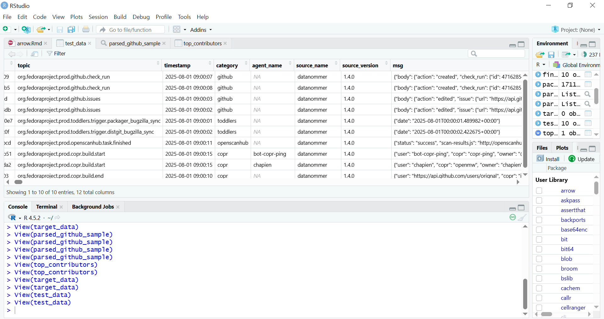
The specific dataset chosen, Datanommer (Fedora Messaging Streams), aligns with the strategic objectives of the Fedora Data Working Group, where I contribute. The data is stored in the Bronze Data Layer where raw data from source systems is ingested and stored, as-is, for scalable data lake storage. The Bronze Layer allows for schema evolution without breaking downstream processes.

To provide the Working Group with transparent access and initial insight into this data, I have prepared a shared Initial Exploratory Data Analysis (EDA) Notebook. This notebook serves as the initial public view of the data quality and patterns, and it informed the subsequent architectural decisions for the scalable pipeline I am about to outline.

Given the complexity of the architecture, I will proceed with an outline of the core components, organized by their role in the ELT pipeline:

Data Architecture Diagram: Assisted by Figma ‘Infinite Canvas’

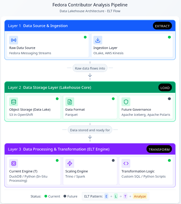
This restructured pipeline, leveraging the new Lakehouse architecture, unlocks several core benefits crucial for scaling contributor analysis and enabling future insights:

Elimination of Memory Constraints via In-Situ Processing

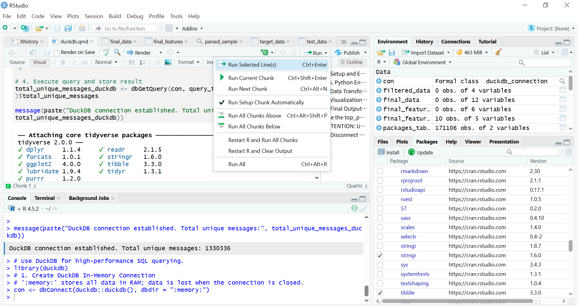
DuckDB acts as a high-performance analytical engine that enables In-Situ Processing. It queries data directly from storage (specifically the Parquet files) without requiring the entire dataset to be loaded into RAM. This not only solves the memory problem but also delivers rapid query execution and significantly lowers operational costs associated with large computational clusters hosted on the OpenShift/Fedora AWS infrastructure.

Quarto runs R code chunks to connect to DuckDB

Future-Proofing

The shift to a Lakehouse model ensures the pipeline is ready for growth and evolving data complexity. Future integration of Apache Iceberg and Apache Polaris will provide schema evolution capabilities. This ensures the pipeline is fully future-proofed against changes in underlying data structures.

Streamlined ELT Workflow and Multi-Lingual Access

I have redefined the processing workflow from a bottlenecked ETL model to a resilient Extract-Load-Transform (ELT) pattern. Parquet files with the variant type store semi-structured data (like JSON/nested structures), loaded raw into S3, simplifies the ingestion stage. When using R, it is recommended to read Parquet files using the Apache Arrow library.

Exploratory Data Analysis (EDA) using data frames in the Tidyverse

The parsed data is then accessible by multiple analytical platforms (R Shiny, Python, BI tools) without duplication or manual preparation. This multi-lingual access maximizes the utility of the clean data layer, supporting a growing number of analytical users and more complex queries necessary for defining long-term contributor metrics.

Initial EDA Notebook

The preliminary Exploratory Data Analysis (EDA) was conducted within the Jupyter Notebook format. This allowed broad compatibility with the existing execution and review environment of the Fedora Data Working Group.

The Initial EDA Notebook is documented to ensure complete reproducibility. This included all necessary steps for the Python library installation and environment setup. Any standard Python script containing ELT logic can be seamlessly run within RStudio’s Python mode or “knitting8” an R Markdown document or rendering a Quarto file.

Conclusion

The establishment of this analysis pipeline represents a crucial step in transforming unprocessed Fedora data into actionable insights. By addressing the core challenges of scaling and in-memory processing through DuckDB, and enabling transparent analysis via the hybrid RStudio/Jupyter workflow, I have demonstrated viable methods for performing Exploratory Data Analysis (EDA) and Extract, Load, Transform (ELT) processes on vast community datasets. In conclusion, the purpose of this work is to foster deeper engagement across a broader community by analyzing data with a view that relates to the Fedora Project community.

I hope this pipeline will serve as the technical foundation that activates and focuses the community discussion around the specific variables and metrics needed to define and ensure the continuity of community contributions.

AI Assistance

The ideation, structural planning, and terminology refinement of the pipelines were assisted by Gemini and Figma.

Software version

RStudio Desktop 2025.05.1 Build 513 (Fedora COPR repository)

R version 4.5.2 (2025-10-31) / Python 3.14.0

Notes

  1. summary(): When used on a data object (for example, DataFrame), it provides basic statistics (min, max, mean, median). When used on a fitted linear model object (lm), it delivers key diagnostic information like coefficient estimates and p-values. ↩
  2. lm(): Stands for Linear Model. This is the core function for fitting linear regression models in R, allowing the user to examine and model the linear relationship between variables. ↩
  3. Regression analysis examines which factors affect the other and which ones are irrelevant for statistical and business context. ↩
  4. DuckDB is a column-oriented database architecture.
    – Direct Querying: It directly queries data from file formats such as Parquet, CSV, and JSON.
    – Local compute engine: It is widely used as a high-performance local compute engine for analytical workloads. It runs in-process, meaning it operates within your application (like a Python script or R session) without needing a separate server or cluster management.
    – Cloud Integration: It supports querying data stored in cloud storage services like AWS S3, GCS (Google Cloud Storage), and Azure Blob Storage.
    ↩
  5. ELT (Extract, Load, Transform): In a modern data environment like a Lakehouse, ELT is preferred: data is first extracted from the source and loaded raw into the cloud data lake (S3), and then transformed in place by the processing engine like DuckDB. ↩
  6. ETL (Extract, Transform, Load): transformations occur before loading the data into the final destination. ↩
  7. Key Advantages of RStudio over Jupyter Notebook for Production Workflows;

    Even with its slightly more complex initial setup compared to Jupyter Notebooks, the advantages become significant when moving from exploration (Jupyter’s strength) to reproducible, production-ready workflows (RStudio’s strength).

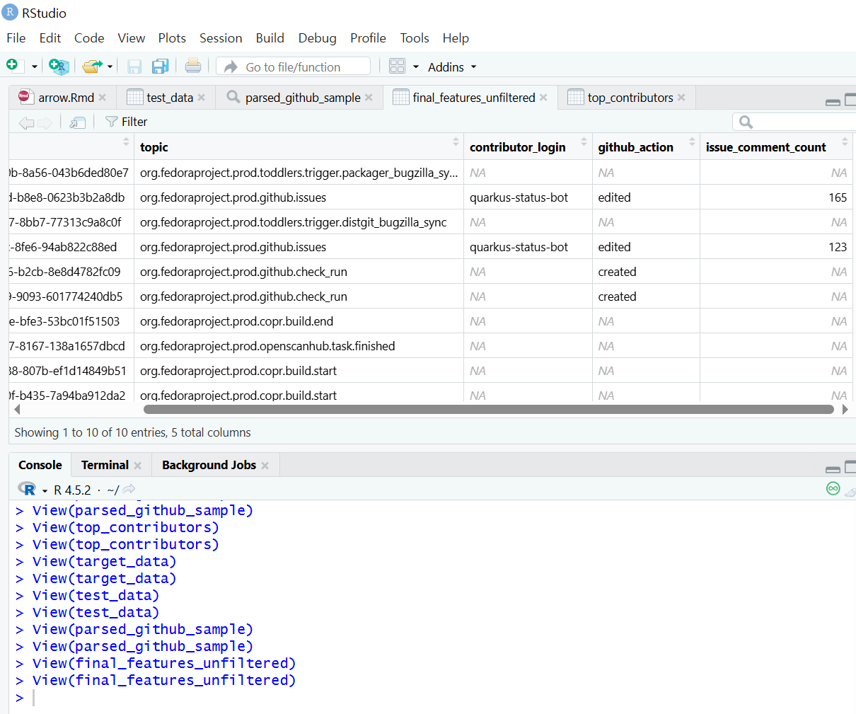
    – Integrated Console, Source, Environment, and Files: RStudio offers a cohesive, four-pane layout that allows for seamless navigation between writing code, running commands, inspecting variables, and managing files/plots. Jupyter requires constant shifting between code cells and external tabs.
    – Superior Debugging Tools: RStudio includes a powerful, visual debugger that allows you to set breakpoints, step through code line-by-line, and inspect variable states directly in the environment pane. Jupyter’s debugging is typically cell-based and less intuitive.
    – Native Project Management: RStudio Projects (.Rproj files) automatically manage the working directory and history. This makes it easy to switch between different analytical tasks without conflicts.
    – Integrated Environment Management (renv): RStudio integrates seamlessly with tools like renv (R Environment) to create isolated, reproducible R environments. This addresses dependency hell by ensuring the exact package versions used in development are used in production, which is crucial for data pipeline version control.
    – Quarto/R Markdown Integration: RStudio provides dedicated tools and buttons for easily compiling and rendering complex analytical documents (like your Quarto file) into HTML, PDF, or presentation slides.
    – Shiny Integration: RStudio is the native environment for developing Shiny web applications—interactive dashboards and tools that turn analysis into deployable products. Jupyter requires separate frameworks (like Dash or Streamlit) for similar deployment.
    – Focus on Scripting: RStudio’s source editor is optimized for writing clean, structured R/Python scripts, which are preferred for building robust, scheduled pipeline components (like those managed by Airflow).
    – Code Chunk Execution (Quarto): Even when using Quarto, RStudio allows for superior navigation and execution of code chunks compared to the often sequential and state-dependent nature of Jupyter Notebook cells. ↩

  8. knitr executes code in R Markdown (.Rmd) file by chunks or as a whole (typically by clicking the “Knit” button in RStudio or using rmarkdown::render() in R) ↩
Posted on Leave a comment

Using data from spreadsheets in Fedora with Python

Python is one of the most popular and powerful programming languages available. Because it’s free and open source, it’s available to everyone — and most Fedora systems come with the language already installed. Python is useful for a wide variety of tasks, but among them is processing comma-separated value (CSV) data. CSV files often start off life as tables or spreadsheets. This article shows how to get started working with CSV data in Python 3.

CSV data is precisely what it sounds like. A CSV file includes one row of data at a time, with data values separated by commas. Each row is defined by the same fields. Short CSV files are often easily read and understood. But longer data files, or those with more fields, may be harder to parse with the naked eye, so computers work better in those cases.

Here’s a simple example where the fields are Name, Email, and Country. In this example, the CSV data includes a field definition as the first row, although that is not always the case.

Name,Email,Country
John Q. Smith,jqsmith@example.com,USA
Petr Novak,pnovak@example.com,CZ
Bernard Jones,bjones@example.com,UK

Reading CSV from spreadsheets

Python helpfully includes a csv module that has functions for reading and writing CSV data. Most spreadsheet applications, both native like Excel or Numbers, and web-based such as Google Sheets, can export CSV data. In fact, many other services that can publish tabular reports will also export as CSV (PayPal for instance).

The Python csv module has a built in reader method called DictReader that can deal with each data row as an ordered dictionary (OrderedDict). It expects a file object to access the CSV data. So if our file above is called example.csv in the current directory, this code snippet is one way to get at this data:

f = open('example.csv', 'r')
from csv import DictReader
d = DictReader(f)
data = []
for row in d: data.append(row)

Now the data object in memory is a list of OrderedDict objects :

[OrderedDict([('Name', 'John Q. Smith'), ('Email', 'jqsmith@example.com'), ('Country', 'USA')]), OrderedDict([('Name', 'Petr Novak'), ('Email', 'pnovak@example.com'), ('Country', 'CZ')]), OrderedDict([('Name', 'Bernard Jones'), ('Email', 'bjones@example.com'), ('Country', 'UK')])]

Referencing each of these objects is easy:

>>> print(data[0]['Country'])
USA
>>> print(data[2]['Email'])
bjones@example.com

By the way, if you have to deal with a CSV file with no header row of field names, the DictReader class lets you define them. In the example above, add the fieldnames argument and pass a sequence of the names:

d = DictReader(f, fieldnames=['Name', 'Email', 'Country'])

A real world example

I recently wanted to pick a random winner from a long list of individuals. The CSV data I pulled from spreadsheets was a simple list of names and email addresses.

Fortunately, Python also has a helpful random module good for generating random values. The randrange function in the Random class from that module was just what I needed. You can give it a regular range of numbers — like integers — and a step value between them. The function then generates a random result, meaning I could get a random integer (or row number!) back within the total number of rows in my data.

So this small program worked well:

from csv import DictReader
from random import Random d = DictReader(open('mydata.csv'))
data = []
for row in d: data.append(row) r = Random()
winner = data[r.randrange(0, len(data), 1)]
print('The winner is:', winner['Name'])
print('Email address:', winner['Email'])

Obviously this example is extremely simple. Spreadsheets themselves include sophisticated ways to analyze data. However, if you want to do something outside the realm of your spreadsheet app, Python may be just the trick!


Photo by Isaac Smith on Unsplash.

Posted on Leave a comment

Best of 2019: Fedora for developers

With the end of the year approaching fast, it is a good time to look back at 2019 and go through the most popular articles on Fedora Magazine written by our contributors.

In this article of the “Best of 2019” series, we are looking at developers and how to use Fedora to be a great developer workstation

Make your Python code look good with Black on Fedora

Black made quite a big impact in the Python ecosystem this year. The project is now part of the Python Software Foundation and it is used by many different projects. So if you write or maintain some Python code and want to stop having to care about code style and code formatting you should check out this article.

How to run virtual machines with virt-manager

Setting up a development environment, running integration tests, testing a new feature, or running an older version of software for all these use cases being able to create and run a virtual machine is a must have knowledge for a developer. This article will walk you through how you can achieve that using virt-manager on your Fedora workstation.

Jupyter and data science in Fedora

With the rise of Data science and machine learning, the Jupyter IDE has become of very popular choice to share or present a program and its results. This article goes into the details of installing and using Jupyter and the different libraries and tools useful for data science.

Building Smaller Container Images

Fedora provides different container images, one of which is a minimal base image. The following article demonstrate how one can use this image to build smaller container images.

Getting Started with Go on Fedora

In 2019 the Go programming language turned 10 year old. In ten years the language has managed to become the default choice for cloud native applications and the cloud ecosystems. Fedora is providing an easy way to start developing in Go, this article takes you through the first step needed to get started.

Stay tuned to the Magazine for other upcoming “Best of 2019” categories. All of us at the Magazine hope you have a great end of year and holiday season.

Posted on Leave a comment

Manage business documents with OpenAS2 on Fedora

Business documents often require special handling. Enter Electronic Document Interchange, or EDI. EDI is more than simply transferring files using email or http (or ftp), because these are documents like orders and invoices. When you send an invoice, you want to be sure that:

1. It goes to the right destination, and is not intercepted by competitors.
2. Your invoice cannot be forged by a 3rd party.
3. Your customer can’t claim in court that they never got the invoice.

The first two goals can be accomplished by HTTPS or email with S/MIME, and in some situations, a simple HTTPS POST to a web API is sufficient. What EDI adds is the last part.

This article does not cover the messy topic of formats for the files exchanged. Even when using a standardized format like ANSI or EDIFACT, it is ultimately up to the business partners. It is not uncommon for business partners to use an ad-hoc CSV file format. This article shows you how to configure Fedora to send and receive in an EDI setup.

Centralized EDI

The traditional solution is to use a Value Added Network, or VAN. The VAN is a central hub that transfers documents between their customers. Most importantly, it keeps a secure record of the documents exchanged that can be used as evidence in disputes. The VAN can use different transfer protocols for each of its customers

AS Protocols and MDN

The AS protocols are a specification for adding a digital signature with optional encryption to an electronic document. What it adds over HTTPS or S/MIME is the Message Disposition Notification, or MDN. The MDN is a signed and dated response that says, in essence, “We got your invoice.” It uses a secure hash to identify the specific document received. This addresses point #3 without involving a third party.

The AS2 protocol uses HTTP or HTTPS for transport. Other AS protocols target FTP and SMTP. AS2 is used by companies big and small to avoid depending on (and paying) a VAN.

OpenAS2

OpenAS2 is an open source Java implemention of the AS2 protocol. It is available in Fedora since 28, and installed with:

$ sudo dnf install openas2
$ cd /etc/openas2

Configuration is done with a text editor, and the config files are in XML. The first order of business before starting OpenAS2 is to change the factory passwords.

Edit /etc/openas2/config.xml and search for ChangeMe. Change those passwords. The default password on the certificate store is testas2, but that doesn’t matter much as anyone who can read the certificate store can read config.xml and get the password.

What to share with AS2 partners

There are 3 things you will exchange with an AS2 peer.

AS2 ID

Don’t bother looking up the official AS2 standard for legal AS2 IDs. While OpenAS2 implements the standard, your partners will likely be using a proprietary product which doesn’t. While AS2 allows much longer IDs, many implementations break with more than 16 characters. Using otherwise legal AS2 ID chars like ‘:’ that can appear as path separators on a proprietary OS is also a problem. Restrict your AS2 ID to upper and lower case alpha, digits, and ‘_’ with no more than 16 characters.

SSL certificate

For real use, you will want to generate a certificate with SHA256 and RSA. OpenAS2 ships with two factory certs to play with. Don’t use these for anything real, obviously. The certificate file is in PKCS12 format. Java ships with keytool which can maintain your PKCS12 “keystore,” as Java calls it. This article skips using openssl to generate keys and certificates. Simply note that sudo keytool -list -keystore as2_certs.p12 will list the two factory practice certs.

AS2 URL

This is an HTTP URL that will access your OpenAS2 instance. HTTPS is also supported, but is redundant. To use it you have to uncomment the https module configuration in config.xml, and supply a certificate signed by a public CA. This requires another article and is entirely unnecessary here.

By default, OpenAS2 listens on 10080 for HTTP and 10443 for HTTPS. OpenAS2 can talk to itself, so it ships with two partnerships using http://localhost:10080 as the AS2 URL. If you don’t find this a convincing demo, and can install a second instance (on a VM, for instance), you can use private IPs for the AS2 URLs. Or install Cjdns to get IPv6 mesh addresses that can be used anywhere, resulting in AS2 URLs like http://[fcbf:fc54:e597:7354:8250:2b2e:95e6:d6ba]:10080.

Most businesses will also want a list of IPs to add to their firewall. This is actually bad practice. An AS2 server has the same security risk as a web server, meaning you should isolate it in a VM or container. Also, the difficulty of keeping mutual lists of IPs up to date grows with the list of partners. The AS2 server rejects requests not signed by a configured partner.

OpenAS2 Partners

With that in mind, open partnerships.xml in your editor. At the top is a list of “partners.” Each partner has a name (referenced by the partnerships below as “sender” or “receiver”), AS2 ID, certificate, and email. You need a partner definition for yourself and those you exchange documents with. You can define multiple partners for yourself. OpenAS2 ships with two partners, OpenAS2A and OpenAS2B, which you’ll use to send a test document.

OpenAS2 Partnerships

Next is a list of “partnerships,” one for each direction. Each partnership configuration includes the sender, receiver, and the AS2 URL used to send the documents. By default, partnerships use synchronous MDN. The MDN is returned on the same HTTP transaction. You could uncomment the as2_receipt_option for asynchronous MDN, which is sent some time later. Use synchronous MDN whenever possible, as tracking pending MDNs adds complexity to your application.

The other partnership options select encryption, signature hash, and other protocol options. A fully implemented AS2 receiver can handle any combination of options, but AS2 partners may have incomplete implementations or policy requirements. For example, DES3 is a comparatively weak encryption algorithm, and may not be acceptable. It is the default because it is almost universally implemented.

If you went to the trouble to set up a second physical or virtual machine for this test, designate one as OpenAS2A and the other as OpenAS2B. Modify the as2_url on the OpenAS2A-to-OpenAS2B partnership to use the IP (or hostname) of OpenAS2B, and vice versa for the OpenAS2B-to-OpenAS2A partnership. Unless they are using the FedoraWorkstation firewall profile, on both machines you’ll need:

# sudo firewall-cmd --zone=public --add-port=10080/tcp

Now start the openas2 service (on both machines if needed):

# sudo systemctl start openas2

Resetting the MDN password

This initializes the MDN log database with the factory password, not the one you changed it to. This is a packaging bug to be fixed in the next release. To avoid frustration, here’s how to change the h2 database password:

$ sudo systemctl stop openas2
$ cat >h2passwd <<'DONE'
#!/bin/bash
AS2DIR="/var/lib/openas2"
java -cp "$AS2DIR"/lib/h2* org.h2.tools.Shell \
-url jdbc:h2:"$AS2DIR"/db/openas2 \
-user sa -password "$1" <<EOF
alter user sa set password '$2';
exit
EOF
DONE
$ sudo sh h2passwd ChangeMe yournewpasswordsetabove
$ sudo systemctl start openas2

Testing the setup

With that out of the way, let’s send a document. Assuming you are on OpenAS2A machine:

$ cat >testdoc <<'DONE'
This is not a real EDI format, but is nevertheless a document.
DONE
$ sudo chown openas2 testdoc
$ sudo mv testdoc /var/spool/openas2/toOpenAS2B
$ sudo journalctl -f -u openas2
... log output of sending file, Control-C to stop following log
^C

OpenAS2 does not send a document until it is writable by the openas2 user or group. As a consequence, your actual business application will copy, or generate in place, the document. Then it changes the group or permissions to send it on its way, to avoid sending a partial document.

Now, on the OpenAS2B machine, /var/spool/openas2/OpenAS2A_OID-OpenAS2B_OID/inbox shows the message received. That should get you started!


Photo by Beatriz Pérez Moya on Unsplash.