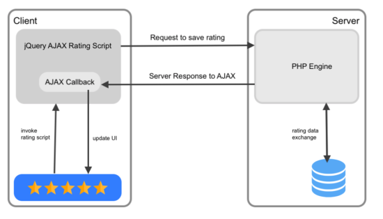
I’m delighted to share an update of Experimental Mobile Blazor Bindings with several new features and fixes. On January 14th we announced the first experimental release of Mobile Blazor Bindings, which enables developers to use familiar web programming patterns to build native mobile apps using C# and .NET for iOS and Android.
Here’s what’s new in this release:
New BoxView, CheckBox, ImageButton, ProgressBar, and Slider components
Xamarin.Essentials is included in the project template
Several properties, events, and other APIs were added to existing components
Made it easier to get from a Blazor component reference to the Xamarin.Forms control
Several bug fixes, including iOS startup
Get started
To get started with Experimental Mobile Blazor Bindings preview 2, install the .NET Core 3.1 SDK and then run the following command:
dotnet new -i Microsoft.MobileBlazorBindings.Templates::0.2.42-preview
And then create your first project by running this command:
dotnet new mobileblazorbindings -o MyApp
That’s it! You can find additional docs and tutorials on https://docs.microsoft.com/mobile-blazor-bindings/.
Upgrade an existing project
To update an existing Mobile Blazor Bindings Preview 1 project to Preview 2 you’ll need to update the Mobile Blazor Bindings NuGet packages to 0.2.42-preview. In each project file (.csproj) update the Microsoft.MobileBlazorBindings package reference’s Version attribute to 0.2.42-preview.
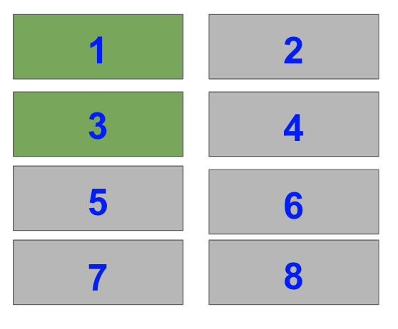
New BoxView, CheckBox, ImageButton, ProgressBar, and Slider components have been added. A picture is worth a thousand words, so here are the new components in action:
And instead of a thousand words, here’s the code for that UI page:
Xamarin.Essentials is included in the project template
Xamarin.Essentials provides developers with cross-platform APIs for their mobile applications. With these APIs you can make cross-platform calls to get geolocation info, get device status and capabilities, access the clipboard, and much more.
Here’s how to get battery status and location information:
Several properties, events, and other APIs were added to existing components
The set of properties available on the default components in Mobile Blazor Bindings now match the Xamarin.Forms UI controls more closely.
For example:
Button events were added: OnPress, OnRelease
Button properties were added: FontSize, ImageSource, Padding, and many more
Label properties were added: MaxLines, Padding, and many more
MenuItem property was added: IsEnabled
NavigableElement property was added: class
And many more!
Made it easier to get from a Blazor component reference to the Xamarin.Forms control
While most UI work is done directly with the Blazor components, some UI functionality is performed by accessing the Xamarin.Forms control. For example, Xamarin.Forms controls have rich animation capabilities that can be accessed via the control itself, such as rotation, fading, scaling, and translation.
To access the Xamarin.Forms element you need to:
Define a field of the type of the Blazor component. For example: Microsoft.MobileBlazorBindings.Elements.Label counterLabel;
Associate the field with a reference to the Blazor component. For example: <label @ref="counterLabel" …></label>
Access the native control via the NativeControl property. For example: await counterLabel.NativeControl.RelRotateTo(360);
Here’s a full example of how to do a rotation animation every time a button is clicked:
Fix src work if NETCore3.0 not installed #55 by 0x414c49
Multi-direction support for Visual Element (RTL, LTR) #59 by 0x414c49
Thank you!
What’s next? Let us know what you want!
We’re listening to your feedback, which has been both plentiful and helpful! We’re also fixing bugs and adding new features. Improved CSS support and inline text are two things we’d love to make available soon.
This project will continue to take shape in large part due to your feedback, so please let us know your thoughts at the GitHub repo or fill out the feedback survey.
Your Python app is slow? It’s time for a speed booster! Learn how in this tutorial.
As you read through the article, feel free to watch the explainer video:
Performance Tuning Concepts 101
I could have started this tutorial with a list of tools you can use to speed up your app. But I feel that this would create more harm than good because you’d spend a lot of time setting up the tools and very little time optimizing your performance.
Instead, I’ll take a different approach addressing the critical concepts of performance tuning first.
So, what’s more important than any one tool for performance optimization?
You must understand the universal concepts of performance tuning first.
The good thing is that you’ll be able to apply those concepts in any language and in any application.
The bad thing is that you must change your expectations a bit: I won’t provide you with a magic tool that speeds up your program on the push of a button.
Let’s start with the following list of the most important things to consider when you think you need to optimize your app’s performance:
Premature Optimization Is The Root Of All Evil
Premature optimization is one of the main problems of badly written code. But what is it anyway?
Definition:Premature optimization is the act of spending valuable resources (time, effort, lines of code, simplicity) to optimize code that doesn’t need to get optimized.
There’s no problem with optimized code per se. The problem is just that there’s no such thing as free lunch. If you think you optimize code snippets, what you’re really doing is to trade one variable (e.g. complexity) against another variable (e.g. performance). An example of such an optimization is to add a cache to avoid computing things repeatedly.
The problem is that if you’re doing it blindly, you may not even realize the harm you’re doing. For example, adding 50% more lines of code just to improve execution speed by 0.1% would be a trade-off that will screw up your whole software development process when done repeatedly.
But don’t take my word for it. This is what one of the most famous computer scientists of all times, Donald Knuth, says about premature optimization:
Programmers waste enormous amounts of time thinking about, or worrying about, the speed of noncritical parts of their programs, and these attempts at efficiency actually have a strong negative impact when debugging and maintenance are considered. We should forget about small efficiencies, say about 97 % of the time: premature optimization is the root of all evil.
A good heuristic is to write the most readable code per default. If this leads to an interactive application that’s already fast enough, good. If users of your application start complaining about speed, then take a structured approach to performance optimization, as described in this tutorial.
Action steps:
Make your code as readable and concise as you can.
Use comments and follow the coding standards (e.g. PEP8 in Python).
Ship your application and do user testing.
Is your application too slow? Really? Okay, then do the following:
Jot down the current performance of your app in seconds if you want to optimize for speed or bytes if you want to optimize for memory.
Do not cross this line until you’ve checked off the previous point.
Measure First, Improve Second
What you measure gets improved. The contrary also holds: what you don’t measure, doesn’t get improved.
This principle is a direct consequence of the first principle: “premature optimization is the root of all evil”. Why? Because if you do premature optimization, you optimize before you measure. But you should always only optimize after you have started your measurements. There’s no point in “improving” runtime if you don’t know from which level you want to improve. Maybe your optimization actually increased runtime? Maybe it had no effect at all? You cannot know unless you have started any attempt to optimize with a clear benchmark.
The consequence is to start with the most straightforward, naive (“dumb”) code that’s also easy to read. This is your benchmark. Any optimization or improvement idea must improve upon this benchmark. As soon as you’ve proven—by rigorous measurement—that your optimization improves your benchmark by X% in performance (memory footprint or speed), this becomes your new benchmark.
This way, your guaranteed to improve the performance of your code over time. And you can document, prove, and defend any optimization to your boss, your peer group, or even the scientific community.
Action steps:
You start with the naive solution that’s easy to read. Mostly, the naive solution is very easy to read.
You take the naive solution as benchmark by measuring its performance rigorously.
You document your measurements in a Google Spreadsheet (okay, you can also use Excel).
You come up with alternative code and measure its performance against the benchmark.
If the new code is better (faster, more memory efficient) than the old benchmark, the new code becomes the new benchmark. All subsequent improvements have to beat the new benchmark (otherwise, you throw them away).
Pareto Is King
I know it’s not big news: the 80/20 Pareto principle—named after Italian economist Vilfredo Pareto—is alive and well in performance optimization.
To exemplify this, have a look at my current CPU usage as I’m writing this:
If you plot this in Python, you see the following Pareto-like distribution:
20% of the code requires 80% of the CPU usage (okay, I haven’t really checked if the numbers match but you get the point).
If I wanted to reduce CPU usage on my computer, I just need to close Cortana and Search and—voilà—a significant portion of the CPU load would be gone:
The interesting observation is that even by removing the two most expensive tasks, the plot looks just the same. Now there are two most expensive tasks: Explorer and System.
This leads us to the 1×1 of performance tuning:
Performance optimization is fractal. As soon as you’re done removing the bottleneck, there’s a new bottleneck lurking around. You “just” need to repeatedly remove the bottleneck to get maximal “bang for your buck”.
Action Steps:
Follow the algorithm.
Identify the bottleneck (= the function with highest negative impact on your performance).
Fix the bottleneck.
Repeat.
Algorithmic Optimization Wins
At this point, you’ve already figured out that you need to optimize your code. You have direct user feedback that your application is too slow. Or you have a strong signal (e.g. through Google Analytics) that your slow web app causes a higher than usual bounce rate etc.
You also know where you are now (in seconds or bytes) and where you want to go (in seconds or bytes).
You also know the bottleneck. (This is where the performance profiling tools discussed below come into play.)
Now, you need to figure out how to overcome the bottleneck. The best leverage point for you as a coder is to tune the algorithms and data structures.
Say, you’re working at a financial application. You know your bottleneck is the function calculate_ROI() that goes over all combinations of potential buying and selling points to calculate the maximum profit (the naive solution). As this is the bottleneck of the whole application, your first task is to find a better algorithm. Fortunately, you find the maximum profit algorithm. The computational complexity reduces from O(n**2) to O(n log n).
(If this particular topic interests you, start reading this SO article.)
Action steps:
Given your current bottleneck function.
Can you improve its data structures? Often, there’s a low hanging fruit by using sets instead of lists (e.g., checking membership is much faster for sets than lists), or dictionaries instead of collections of tuples.
Can you find better algorithms that are already proven? Can you tweak existing algorithms for your specific problem at hand?
Spend a lot of time researching these questions. It pays off. You’ll become a better computer scientist in the process. And it’s your bottleneck after all—so it’s a huge leverage point for your application.
All Hail to the Cache
Have you checked off all previous boxes? You know exactly where you are and where you want to go. You know what bottleneck to optimize. You know about alternative algorithms and data structures.
Here’s a quick and dirty trick that works surprisingly well for a large variety of applications. To improve your performance often means to remove unnecessary computations. One low-hanging fruit is to store the result of a subset of computations you have already performed in a cache.
How can you create a cache in practice? In Python, it’s as simple as creating a dictionary where you associate each function input (e.g. as an input string) with the function output.
You can then ask the cache to give you the computations you’ve already performed.
A simple example of an effective use of caching (sometimes called memoization) is the Fibonacci algorithm:
def fib2(n): if n<2: return n return fib2(n-1) + fib2(n-2)
The problem is that the function calls fib2(n-1) and fib2(n-2) calculate largely the same things. For instance, both separately calculate the Fibonacci value fib2(n-3). This adds up!
But with caching, you can simply memorize the results of previous computations so that the result for fib2(n-3) is calculated only once. All other times, you can pull the result from the cache and get an instant result.
Here’s the caching variant of Python Fibonacci:
def fib(n): if n in cache: return cache[n] if n < 2: return n fib_n = fib(n-1) + fib(n-2) cache[n] = fib_n return fib_n
You store the result of the computation fib(n-1) + fib(n-2) in the cache. If you already have the result of the n-th Fibonacci number, you simply pull it from the cache rather than recalculating it again and again.
Here’s the surprising speed improvement—just by using a simple cache:
import time t1 = time.time()
print(fib2(40))
t2 = time.time()
print(fib(40))
t3 = time.time() print("Fibonacci without cache: " + str(t2-t1))
print("Fibonacci with cache: " + str(t3-t2)) ''' OUTPUT:
102334155
102334155
Fibonacci without cache: 31.577041387557983
Fibonacci with cache: 0.015461206436157227 '''
There are two basic strategies you can use:
Perform computations in advanced (“offline”) and store their results in the cache. This is a great strategy for web applications where you can fill up a large cache once (or once a day) and then simply serve the result of your precomputations to the users. For them, your calculations “feel” blazingly fast. But in reality, you just serve them precalculated values. Google Maps heavily uses this trick to speedup shortest path computations.
Perform computations as they appear (“online”) and store their results in the cache. This reactive form is the most basic and simplest form of caching where you don’t need to decide which computations to perform in advance.
In both cases, the more computations you store, the higher the likelihood of “cache hits” where the computation can be returned immediately. But as you usually have a memory limit (e.g. 100,000 cache entries), you need to decide about a sensible cache replacement policy.
Action steps:
Think: How can you reduce redundant computations? Would caching be a sensible approach?
What type of data / computations do you cache?
What’s the size of your cache?
Which entries to remove if the cache is full?
If you have a web application, can you reuse computations of previous users to compute the result of your current user?
Less is More
Your problem is too hard? Make it easier!
Yes, it’s obvious. But then again, so many coders are too perfectionistic about their code. They accept huge complexity and computational overhead—just for this small additional feature that often doesn’t even get recognized by users.
A powerful “trick” for performance optimization is to seek out easier problems. Instead of spending your effort optimizing, it’s often much better to get rid of complexity, unnecessary features and computations, data. Use heuristics rather than optimal algorithms wherever possible. You often pay for perfect results with a 10x slow down in performance.
So ask yourself this: what is your current bottleneck function really doing? Is it really worth the effort? Can you remove the feature or offer a down-sized version? If the feature is used by 1% of your users but 100% perceive the increased latency, it may be time for some minimalism!
Action step:
Can you remove your current bottleneck altogether by just skipping the feature?
Can you simplify the problem?
Think 80/20: get rid of one expensive feature to add 10 non-expensive ones.
Think opportunity costs: omit one important feature so that you can pursue a very important feature.
Know When to Stop
It’s easy to do but it’s also easy not to do: stop!
Performance optimization can be one of the most time-intensive things to do as a coder. There’s always room for improvement. You can always tweak and improve. But your effort to improve your performance by X increases superlinearly or even exponentially to X. At some point, it’s just a waste of your time of improving your performance.
Action step:
Ask yourself constantly: is it really worth the effort to keep optimizing?
Python Profilers
Python comes with different profilers. If you’re new to performance optimization, you may ask: what’s a profiler anyway?
A performance profiler allows you to monitor your application more closely. If you just run a Python script in your shell, you see nothing but the output produced by your program. But you don’t see how much bytes were consumed by your program. You don’t see how long each function runs. You don’t see the data structures that caused most memory overhead.
Without those things, you cannot know what’s the bottleneck of your application. And, as you’ve already learned above, you cannot possibly start optimizing your code. Why? Because else you were complicit in “premature optimization”—one of the deadly sins in programming.
Instrumenting profilers insert special code at the beginning and end of each routine to record when the routine starts and when it exits. With this information, the profiler aims to measure the actual time taken by the routine on each call. This type of profiler may also record which other routines are called from a routine. It can then display the time for the entire routine and also break it down into time spent locally and time spent on each call to another routine.
Fortunately, there are a lot of profilers. In the remaining article, I’ll give you an overview of the most important profilers in Python and how to use them. Each comes with a reference for further reading.
Python cProfile
The most popular Python profiler is called cProfile. You can import it much like any other library by using the statement:
import cProfile
A simple statement but nonetheless a powerful tool in your toolbox.
Let’s write a Python script which you can profile. Say, you come up with this (very) raw Python script to find 100 random prime numbers between 2 and 1000 which you want to optimize:
import random def guess(): ''' Returns a random number ''' return random.randint(2, 1000) def is_prime(x): ''' Checks whether x is prime ''' for i in range(x): for j in range(x): if i * j == x: return False return True def find_primes(num): primes = [] for i in range(num): p = guess() while not is_prime(p): p = guess() primes += [p] return primes print(find_primes(100)) '''
[733, 379, 97, 557, 773, 257, 3, 443, 13, 547, 839, 881, 997,
431, 7, 397, 911, 911, 563, 443, 877, 269, 947, 347, 431, 673,
467, 853, 163, 443, 541, 137, 229, 941, 739, 709, 251, 673, 613,
23, 307, 61, 647, 191, 887, 827, 277, 389, 613, 877, 109, 227,
701, 647, 599, 787, 139, 937, 311, 617, 233, 71, 929, 857, 599,
2, 139, 761, 389, 2, 523, 199, 653, 577, 211, 601, 617, 419, 241,
179, 233, 443, 271, 193, 839, 401, 673, 389, 433, 607, 2, 389,
571, 593, 877, 967, 131, 47, 97, 443] '''
The program is slow (and you sense that there are many optimizations). But where to start?
As you’ve already learned, you need to know the bottleneck of your script. Let’s use the cProfile module to find it! The only thing you need to do is to add the following two lines to your script:
It’s really that simple. First, you write your script. Second, you call the cProfile.run() method to analyze its performance. Of course, you need to replace the execution command with your specific code you want to analyze. For example, if you want to test function f42(), you need to type in cProfile.run('f42()').
Here’s the output of the previous code snippet (don’t panic yet):
It still gives you the output to the shell—even if you didn’t execute the code directly, the cProfile.run() function did. You can see the list of the 100 random prime numbers here.
The next part prints some statistics to the shell:
3908 function calls in 1.614 seconds
Okay, this is interesting: the whole program took 1.614 seconds to execute. In total, 3908 function calls have been executed. Can you figure out which?
The print() function once.
The find_primes(100) function once.
The find_primes() function executes the for loop 100 times.
In the for loop, we execute the range(), guess(), and is_prime() functions. The program executes the guess() and is_prime() functions multiple times per loop iteration until it correctly guessed the next prime number.
The guess() function executes the randint(2,1000) method once.
The next part of the output shows you the detailed stats of the function names ordered by the function name (not its performance):
Each line stands for one function. For example the second line stands for the function is_prime. You can see that is_prime() had 535 executions with a total time of 1.54 seconds.
Wow! You’ve just found the bottleneck of the whole program: is_prime(). Again, the total execution time was 1.614 seconds and this one function dominates 95% of the total execution time!
So, you need to ask yourself the following questions: Do you need to optimize the code at all? If you do, how can you mitigate the bottleneck?
There are two basic ideas:
call the function is_prime() less frequently, and
optimize performance of the function itself.
You know that the best way to optimize code is to look for more efficient algorithms. A quick search reveals a much more efficient algorithm (see function is_prime2()).
import random def guess(): ''' Returns a random number ''' return random.randint(2, 1000) def is_prime(x): ''' Checks whether x is prime ''' for i in range(x): for j in range(x): if i * j == x: return False return True def is_prime2(x): ''' Checks whether x is prime ''' for i in range(2,int(x**0.5)+1): if x % i == 0: return False return True def find_primes(num): primes = [] for i in range(num): p = guess() while not is_prime2(p): p = guess() primes += [p] return primes import cProfile
cProfile.run('print(find_primes(100))')
What do you think: is our new prime checker faster? Let’s study the output of our code snippet:
Crazy – what a performance improvement! With the old bottleneck, the code takes 1.6 seconds. Now, it takes only 0.074 seconds—a 95% runtime performance improvement!
That’s the power of bottleneck analysis.
The cProfile method has many more functions and parameters but this simple method cProfile.run() is already enough to resolve many performance bottlenecks.
How to Sort the Output of the cProfile.run() Method?
To sort the output with respect to the i-th column, you can pass the sort=i argument to the cProfile.run() method. Here’s the help output:
>>> import cProfile
>>> help(cProfile.run)
Help on function run in module cProfile: run(statement, filename=None, sort=-1) Run statement under profiler optionally saving results in filename This function takes a single argument that can be passed to the "exec" statement, and an optional file name. In all cases this routine attempts to "exec" its first argument and gather profiling statistics from the execution. If no file name is present, then this function automatically prints a simple profiling report, sorted by the standard name string (file/line/function-name) that is presented in each line.
And here’s a minimal example profiling the above find_prime() method:
If you’re running a flask application on a server, you often want to improve performance. But remember: you must focus on the bottlenecks of your whole application—not only the performance of the Flask app running on your server. There are many other possible performance bottlenecks such as database access, heavy use of images, wrong file formats, videos, embedded scripts, etc.
Before you start optimizing the Flask app itself, you should first check out those speed analysis tools that analyze the end-to-end latency as perceived by the user.
These online tools are free and easy to use: you just have to copy&paste the URL of your website and press a button. They will then point you to the potential bottlenecks of your app. Just run all of them and collect the results in an excel file or so. Then spend some time thinking about the possible bottlenecks until your pretty confident that you’ve found the main bottleneck.
Here’s an example of a Google Page Speed run for the wealth creation Flask app www.wealthdashboard.app:
It’s clear that in this case, the performance bottleneck is the work performed by the application itself. This doesn’t surprise as it comes with rich and interactive user interface:
So in this case, it makes absolutely sense to dive into the Python Flask app itself which, in turn, uses the dash framework as a user interface.
So let’s start with the minimal example of the dash app. Note that the dash app internally runs a Flask server:
import dash
import dash_core_components as dcc
import dash_html_components as html external_stylesheets = ['https://codepen.io/chriddyp/pen/bWLwgP.css'] app = dash.Dash(__name__, external_stylesheets=external_stylesheets) app.layout = html.Div(children=[ html.H1(children='Hello Dash'), html.Div(children=''' Dash: A web application framework for Python. '''), dcc.Graph( id='example-graph', figure={ 'data': [ {'x': [1, 2, 3], 'y': [4, 1, 2], 'type': 'bar', 'name': 'SF'}, {'x': [1, 2, 3], 'y': [2, 4, 5], 'type': 'bar', 'name': u'Montréal'}, ], 'layout': { 'title': 'Dash Data Visualization' } } )
]) if __name__ == '__main__': #app.run_server(debug=True) import cProfile cProfile.run('app.run_server(debug=True)', sort=1)
Don’t worry, you don’t need to understand what’s going on. Only one thing is important: rather than running app.run_server(debut=True) in the third last line, you execute the cProfile.run(...) wrapper. You sort the output with respect to decreasing runtime (second column). The result of executing and terminating the Flask app looks as follows:
So there have been 6031 function calls—but runtime was dominated by the method WaitForSingleObject() as you can see in the first row of the output table. This makes sense as I only ran the server and shut it down—it didn’t really process any request.
But if you’d execute many requests as you test your server, you’d quickly find out about the bottleneck methods.
There are some specific profilers for Flask applications. I’d recommend that you start looking here:
You can set up the profiler in just a few lines of code. However, this flask profiler focuses on the performance of multiple endpoints (“urls”). If you want to explore the function calls of a single endpoint/url, you should still use the cProfile module for fine-grained analysis.
An easy way of using the cProfile module in your flask application is the Werkzeug project. Using it is as simple as wrapping the flask app like this:
from werkzeug.contrib.profiler import ProfilerMiddleware
app = ProfilerMiddleware(app)
Per default, the profiled data will be printed to your shell or the standard output (depends on how you serve your Flask application).
Pandas Profiling Example
To profile your pandas application, you should divide your overall script into many functions and use Python’s cProfile module (see above). This will quickly point towards potential bottlenecks.
However, if you want to find out about a specific Pandas dataframe, you could use the following two methods:
You’ve learned how to approach the problem of performance optimization conceptually:
Premature Optimization Is The Root Of All Evil
Measure First, Improve Second
Pareto Is King
Algorithmic Optimization Wins
All Hail to the Cache
Less is More
Know When to Stop
These concepts are vital for your coding productivity—they can save you weeks, if not months of mindless optimization.
The most important principle is to always focus on resolving the next bottleneck.
You’ve also learned about Python’s powerful cProfile module that helps you spot performance bottlenecks quickly. For the vast majority of Python applications, including Flask and Pandas, this will help you figure out the most critical bottlenecks.
Most of the time, there’s no need to optimize, say, beyond the first three bottlenecks (exception: scientific computing).
Python comes with different profilers. If you’re new to performance optimization, you may ask: what’s a profiler anyway?
A performance profiler allows you to monitor your application more closely. If you just run a Python script in your shell, you see nothing but the output produced by your program. But you don’t see how much bytes were consumed by your program. You don’t see how long each function runs. You don’t see the data structures that caused most memory overhead.
Without those things, you cannot know what’s the bottleneck of your application. And, as you’ve already learned above, you cannot possibly start optimizing your code. Why? Because else you were complicit in “premature optimization”—one of the deadly sins in programming.
Instrumenting profilers insert special code at the beginning and end of each routine to record when the routine starts and when it exits. With this information, the profiler aims to measure the actual time taken by the routine on each call. This type of profiler may also record which other routines are called from a routine. It can then display the time for the entire routine and also break it down into time spent locally and time spent on each call to another routine.
Fortunately, there are a lot of profilers. In the remaining article, I’ll give you an overview of the most important profilers in Python and how to use them. Each comes with a reference for further reading.
Python cProfile
The most popular Python profiler is called cProfile. You can import it much like any other library by using the statement:
import cProfile
A simple statement but nonetheless a powerful tool in your toolbox.
Let’s write a Python script which you can profile. Say, you come up with this (very) raw Python script to find 100 random prime numbers between 2 and 1000 which you want to optimize:
import random def guess(): ''' Returns a random number ''' return random.randint(2, 1000) def is_prime(x): ''' Checks whether x is prime ''' for i in range(x): for j in range(x): if i * j == x: return False return True def find_primes(num): primes = [] for i in range(num): p = guess() while not is_prime(p): p = guess() primes += [p] return primes print(find_primes(100)) '''
[733, 379, 97, 557, 773, 257, 3, 443, 13, 547, 839, 881, 997,
431, 7, 397, 911, 911, 563, 443, 877, 269, 947, 347, 431, 673,
467, 853, 163, 443, 541, 137, 229, 941, 739, 709, 251, 673, 613,
23, 307, 61, 647, 191, 887, 827, 277, 389, 613, 877, 109, 227,
701, 647, 599, 787, 139, 937, 311, 617, 233, 71, 929, 857, 599,
2, 139, 761, 389, 2, 523, 199, 653, 577, 211, 601, 617, 419, 241,
179, 233, 443, 271, 193, 839, 401, 673, 389, 433, 607, 2, 389,
571, 593, 877, 967, 131, 47, 97, 443] '''
The program is slow (and you sense that there are many optimizations). But where to start?
As you’ve already learned, you need to know the bottleneck of your script. Let’s use the cProfile module to find it! The only thing you need to do is to add the following two lines to your script:
It’s really that simple. First, you write your script. Second, you call the cProfile.run() method to analyze its performance. Of course, you need to replace the execution command with your specific code you want to analyze. For example, if you want to test function f42(), you need to type in cProfile.run('f42()').
Here’s the output of the previous code snippet (don’t panic yet):
It still gives you the output to the shell—even if you didn’t execute the code directly, the cProfile.run() function did. You can see the list of the 100 random prime numbers here.
The next part prints some statistics to the shell:
3908 function calls in 1.614 seconds
Okay, this is interesting: the whole program took 1.614 seconds to execute. In total, 3908 function calls have been executed. Can you figure out which?
The print() function once.
The find_primes(100) function once.
The find_primes() function executes the for loop 100 times.
In the for loop, we execute the range(), guess(), and is_prime() functions. The program executes the guess() and is_prime() functions multiple times per loop iteration until it correctly guessed the next prime number.
The guess() function executes the randint(2,1000) method once.
The next part of the output shows you the detailed stats of the function names ordered by the function name (not its performance):
Each line stands for one function. For example the second line stands for the function is_prime. You can see that is_prime() had 535 executions with a total time of 1.54 seconds.
Wow! You’ve just found the bottleneck of the whole program: is_prime(). Again, the total execution time was 1.614 seconds and this one function dominates 95% of the total execution time!
So, you need to ask yourself the following questions: Do you need to optimize the code at all? If you do, how can you mitigate the bottleneck?
There are two basic ideas:
call the function is_prime() less frequently, and
optimize performance of the function itself.
You know that the best way to optimize code is to look for more efficient algorithms. A quick search reveals a much more efficient algorithm (see function is_prime2()).
import random def guess(): ''' Returns a random number ''' return random.randint(2, 1000) def is_prime(x): ''' Checks whether x is prime ''' for i in range(x): for j in range(x): if i * j == x: return False return True def is_prime2(x): ''' Checks whether x is prime ''' for i in range(2,int(x**0.5)+1): if x % i == 0: return False return True def find_primes(num): primes = [] for i in range(num): p = guess() while not is_prime2(p): p = guess() primes += [p] return primes import cProfile
cProfile.run('print(find_primes(100))')
What do you think: is our new prime checker faster? Let’s study the output of our code snippet:
Crazy – what a performance improvement! With the old bottleneck, the code takes 1.6 seconds. Now, it takes only 0.074 seconds—a 95% runtime performance improvement!
You’ve learned how to use the cProfile module in Python to find the bottleneck of your application.
If you’re already optimizing performance of your Python apps, chances are that you can already earn six figures by selling your Python skills. Would you like to learn how?
Join the free webinar that shows you how to become a thriving coding business owner online!
Too much stuff happening in a single plot? No problem—use multiple subplots!
This in-depth tutorial shows you everything you need to know to get started with Matplotlib’s subplot() function.
If you want, just hit “play” and watch the explainer video. I’ll then guide you through the tutorial:
To create a matplotlib subplot with any number of rows and columns, use the plt.subplot() function.
It takes 3 arguments, all of which are integers and positional only i.e. you cannot use keywords to specify them.
plt.subplot(nrows, ncols, index)
nrows – the number of rows
ncols – the number of columns
index – the Subplot you want to select (starting from 1 in the top left)
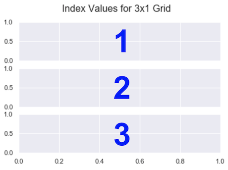
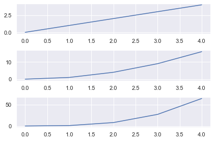
So, plt.subplot(3, 1, 1) has 3 rows, 1 column (a 3 x 1 grid) and selects Subplot with index 1.
After plt.subplot(), code your plot as normal using the plt. functions you know and love. Then, select the next subplot by increasing the index by 1 – plt.subplot(3, 1, 2) selects the second Subplot in a 3 x 1 grid. Once all Subplots have been plotted, call plt.tight_layout() to ensure no parts of the plots overlap. Finally, call plt.show() to display your plot.
# Import necessary modules and (optionally) set Seaborn style
import matplotlib.pyplot as plt
import seaborn as sns; sns.set()
import numpy as np # Generate data to plot
linear = [x for x in range(5)]
square = [x**2 for x in range(5)]
cube = [x**3 for x in range(5)] # 3x1 grid, first subplot
plt.subplot(3, 1, 1)
plt.plot(linear) # 3x1 grid, second subplot
plt.subplot(3, 1, 2)
plt.plot(square) # 3x1 grid, third subplot
plt.subplot(3, 1, 3)
plt.plot(cube) plt.tight_layout()
plt.show()
Matplotlib Subplot Example
The arguments for plt.subplot() are intuitive:
plt.subplot(nrows, ncols, index)
The first two – nrows and ncols – stand for the number of rows and number of columns respectively.
If you want a 2×2 grid, set nrows=2 and ncols=2. For a 3×1 grid, it’s nrows=3 and ncols=1.
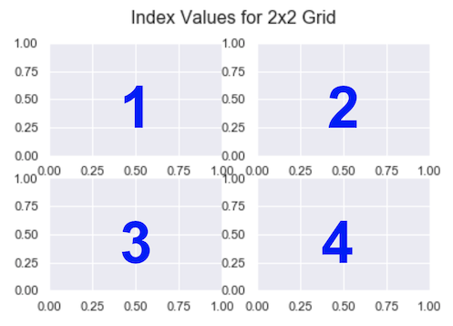
The index is the subplot you want to select. The code you write immediately after it is drawn on that subplot. Unlike everything else in the Python universe, indexing starts from 1, not 0. It continues from left-to-right in the same way you read.
So, for a 2 x 2 grid, the indexes are
For a 3 x 1 grid, they are
The arguments for plt.subplot() are positional only. You cannot pass them as keyword arguments.
>>> plt.subplot(nrows=3, ncols=1, index=1)
AttributeError: 'AxesSubplot' object has no property 'nrows'
However, the comma between the values is optional, if each value is an integer less than 10.
Thus, the following are equivalent – they both select index 1 from a 3×1 grid.
plt.subplot(3, 1, 1)
plt.subplot(311)
I will alternate between including and excluding commas to aid your learning.
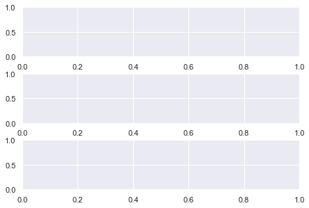
Let’s look at the default subplot layout and the general outline for your code.
plt.subplot(3, 1, 1)
<em># First subplot here</em> plt.subplot(3, 1, 2)
<em># Second subplot here</em> plt.subplot(3, 1, 3)
<em># Third subplot here</em> plt.show()
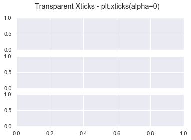
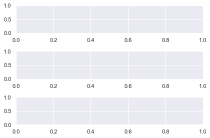
This looks ok but the x-axis labels are hard to read on the top 2 subplots.
You have a few ways to solve this problem.
First, you can manually adjust the xticks with the matplotlib xticks function – plt.xticks() – and either:
make them transparent by setting alpha=0, or
move them and decrease their font size with the position and size arguments
# Make xticks of top 2 subplots transparent
plt.subplot(3, 1, 1)
plt.xticks(alpha=0) plt.subplot(3, 1, 2)
plt.xticks(alpha=0) # Plot nothing on final subplot
plt.subplot(3, 1, 3) plt.suptitle('Transparent Xticks - plt.xticks(alpha=0)')
plt.show()
# Move and decrease size of xticks on all subplots
plt.subplot(3, 1, 1)
plt.xticks(position=(0, 0.1), size=10) plt.subplot(3, 1, 2)
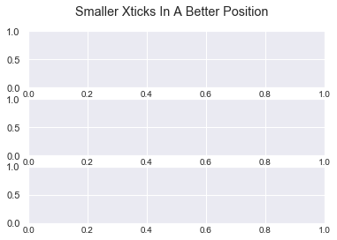
plt.xticks(position=(0, 0.1), size=10) plt.subplot(3, 1, 3)
plt.xticks(position=(0, 0.1), size=10) plt.suptitle('Smaller Xticks In A Better Position')
plt.show()
Both these methods work but are fiddly. Plus, you cannot automate them which is annoying for us programmers.
You have this ticks problem whenever you create subplots. Thankfully, the matplotlib tight_layout function was created to solve this.
Matplotlib Tight_Layout
By calling plt.tight_layout(), matplotlib automatically adjusts the following parts of the plot to make sure they don’t overlap:
axis labels set with plt.xlabel() and plt.ylabel(),
tick labels set with plt.xticks() and plt.yticks(),
titles set with plt.title() and plt.suptitle()
Note that this feature is experimental. It’s not perfect but often does a really good job. Also, note that it does not work too well with legends or colorbars – you’ll see how to work with them later.
Let’s see the most basic example without any labels or titles.
Now there is plenty of space between the plots. You can adjust this with the pad keyword. It accepts a float in the range [0.0, 1.0] and is a fraction of the font size.
Now there is less space between the plots but everything is still readable. I use plt.tight_layout() in every single plot (without colobars or legends) and I recommend you do as well. It’s an easy way to make your plots look great.
It is the overall window/page that everything is drawn on. You can have multiple independent figures and Figures can contain multiple Subplots
In other words, the Figure is the blank canvas you ‘paint’ all your plots on.
If you are happy with the size of your subplots but you want the final image to be larger/smaller, change the Figure. Do this at the top of your code with the matplotlib figure function – plt.figure().
# Make Figure 3 inches wide and 6 inches long
plt.figure(figsize=(3, 6)) # Create 2x1 grid of subplots
plt.subplot(211)
plt.subplot(212)
plt.show()
Before coding any subplots, call plt.figure() and specify the Figure size with the figsize argument. It accepts a tuple of 2 numbers – (width, height) of the image in inches.
Above, I created a plot 3 inches wide and 6 inches long – plt.figure(figsize=(3, 6)).
# Make a Figure twice as long as it is wide
plt.figure(figsize=plt.figaspect(2)) # Create 2x1 grid of subplots
plt.subplot(211)
plt.subplot(212)
plt.show()
You can set a more general Figure size with the matplotlib figaspect function. It lets you set the aspect ratio (height/width) of the Figure.
Above, I created a Figure twice as long as it is wide by setting figsize=plt.figaspect(2).
Note: Remember the aspect ratio (height/width) formula by recalling that height comes first in the alphabet.
Now let’s look at putting different sized Subplots on one Figure.
Matplotlib Subplots Different Sizes
The hardest part of creating a Figure with different sized Subplots in matplotlib is figuring out what fraction each Subplot takes up.
So, you should know what you are aiming for before you start. You could sketch it on paper or draw shapes in PowerPoint. Once you’ve done this, everything else is much easier.
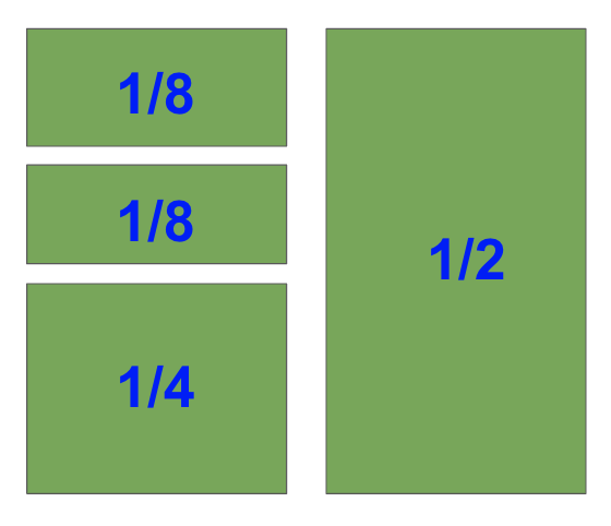
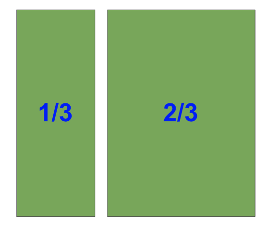
I’m going to create this shape
I’ve labeled the fraction each Subplot takes up as we need this for our plt.subplot() calls.
I’ll create the biggest subplot first and the others in descending order.
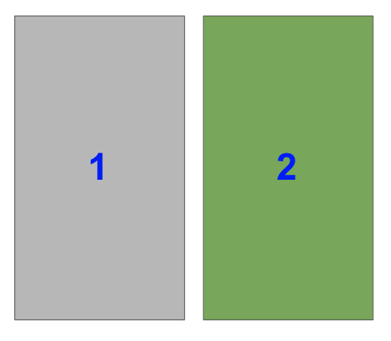
The right-hand side is half of the plot. It is one of two plots on a Figure with 1 row and 2 columns. To select it with plt.subplot(), you need to set index=2.
Note that in the image, the blue numbers are the index values each Subplot has.
In code, this is
plt.subplot(122)
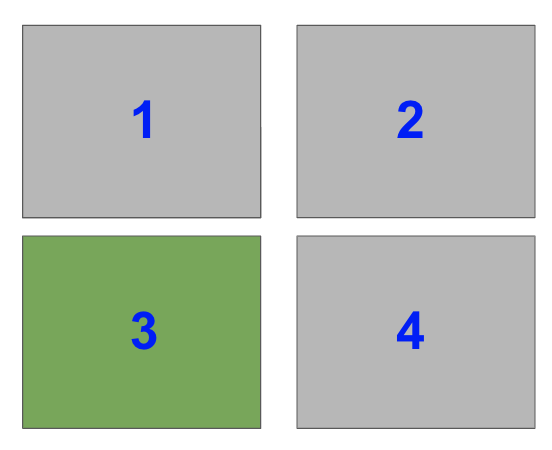
Now, select the bottom left Subplot in a a 2×2 grid i.e. index=3
plt.subplot(223)
Lastly, select the top two Subplots on the left-hand side of a 4×2 grid i.e. index=1 and index=3.
plt.subplot(421)
plt.subplot(423)
When you put this altogether you get
# Subplots you have just figured out
plt.subplot(122)
plt.subplot(223)
plt.subplot(421)
plt.subplot(423) plt.tight_layout(pad=0.1)
plt.show()
Perfect! Breaking the Subplots down into their individual parts and knowing the shape you want makes everything easier.
Matplotlib Subplot Size Different
You may have noticed that each of the Subplots in the previous example took up 1/x fraction of space – 1/2, 1/4 and 1/8.
With the matplotlib subplot function, you can only create Subplots that are 1/x.
It is not possible to create the above plot in matplotlib using the plt.subplot() function. However, if you use the matplotlib subplots function or GridSpec, then it can be done.
Matplotlib Subplots_Adjust
If you aren’t happy with the spacing between plots that plt.tight_layout() provides, manually adjust it with plt.subplots_adjust().
It takes 6 optional, self-explanatory keyword arguments. Each accepts a float in the range [0.0, 1.0] and they are a fraction of the font size:
left, right, bottom and top is the spacing on each side of the Subplot
wspace – the width between Subplots
hspace – the height between Subplots
# Same grid as above
plt.subplot(122)
plt.subplot(223)
plt.subplot(421)
plt.subplot(423) # Set horizontal and vertical space to 0.05
plt.subplots_adjust(hspace=0.05, wspace=0.05)
plt.show()
In this example, I decreased both the height and width to just 0.05. Now there is hardly any space between the plots.
To avoid loads of similar examples, play around with the arguments yourself to get a feel for how this function works.
Matplotlib Suplot DPI
The Dots Per Inch (DPI) is a measure of printer resolution. It is the number of colored dots placed on each square inch of paper when it’s printed. The more dots you have, the higher the quality of the image. If you are going to print your plot on a large poster, it’s a good idea to use a large DPI.
The DPI for each Figure is controlled by the plt.rcParams dictionary. It contains all the runtime configuration settings. If you print plt.rcParams to the screen, you will see all the variables you can modify. We want figure.dpi.
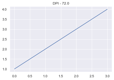
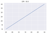
Let’s make a simple line plot first with the default DPI (72.0) and then a much smaller value.
The Figure with a smaller DPI is smaller and has a lower resolution.
If you want to permanently change the DPI of all matplotlib Figures – or any of the runtime configuration settings – find the matplotlibrc file on your system and modify it.
You can find it by entering
import matplotlib as mpl
mpl.matplotlib_fname()
Once you have found it, there are notes inside telling you what everything does.
Matplotlib Subplot Spacing
The function plt.tight_layout() solves most of your spacing issues. If that is not enough, call it with the optional pad and pass a float in the range [0.0, 1.0]. If that still is not enough, use the plt.subplots_adjust() function.
I’ve explained both of these functions in detail further up the article.
Matplotlib Subplot Colorbar
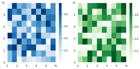
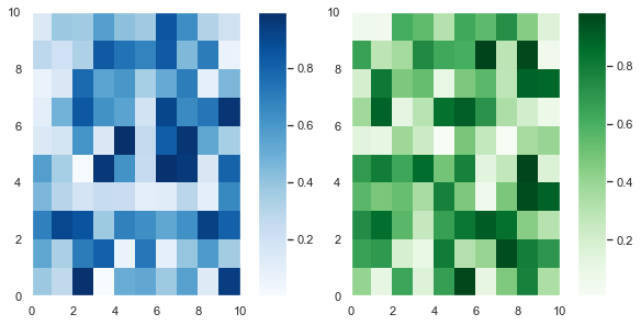
Adding a colorbar to each plot is the same as adding a title – code it underneath the plt.subplot() call you are currently working on. Let’s plot a 1×2 grid where each Subplot is a heatmap of randomly generated numbers.
For more info on the Python random module, check out my article. I use the Numpy random module below but the same ideas apply.
# Set seed so you can reproduce results
np.random.seed(1) # Create a 10x10 array of random floats in the range [0.0, 1.0]
data1 = np.random.random((10, 10))
data2 = np.random.random((10, 10)) # Make figure twice as wide as it is long plt.figure(figsize=plt.figaspect(1/2)) # First subplot
plt.subplot(121)
pcm1 = plt.pcolormesh(data1, cmap='Blues')
plt.colorbar(pcm1) # Second subplot
plt.subplot(122)
pcm2 = plt.pcolormesh(data2, cmap='Greens')
plt.colorbar(pcm2) plt.tight_layout()
plt.show()
First, I created some (10, 10) arrays containing random numbers between 0 and 1 using the np.random.random() function. Then I plotted them as heatmaps using plt.pcolormesh(). I stored the result and passed it to plt.colorbar(), then finished the plot.
As this is an article on Subplots, I won’t discuss the matplotlib pcolormesh function in detail.
Since these plots are different samples of the same data, you can plot them with the same color and just draw one colorbar.
To draw this plot, use the same code as above and set the same colormap in both matplotlib pcolormesh calls – cmap='Blues'. Then draw the colorbar on the second subplot.
This doesn’t look as good as the above Figure since the colorbar takes up space from the second Subplot. Unfortunately, you cannot change this behavior – the colorbar takes up space from the Subplot it is drawn next to.
A Grid is the number of rows and columns you specify when calling plt.subplot(). Each section of the Grid is called a cell. You can create any sized grid you want. But plt.subplot() only creates Subplots that span one cell. To create Subplots that span multiple cells, use the GridSpec class, the plt.subplots() function or the subplot2grid method.
I discuss these in detail in my article on matplotlib subplots.
Summary
Now you know everything there is to know about the subplot function in matplotlib.
You can create grids of any size you want and draw subplots of any size – as long as it takes up 1/xth of the plot. If you want a larger or smaller Figure you can change it with the plt.figure() function. Plus you can control the DPI, spacing and set the title.
Armed with this knowlege, you can now make impressive plots of unlimited complexity.
But you have also discovered some of the limits of the subplot function. And you may feel that it is a bit clunky to type plt.subplot() whenever you want to draw a new one.
To learn how to create more detailed plots with less lines of code, read my article on the plt.subplots() (with an ‘s’) function.
Where To Go From Here?
Do you wish you could be a programmer full-time but don’t know how to start?
Check out my pure value-packed webinar where I teach you to become a Python freelancer in 60 days or your money back!
It doesn’t matter if you’re a Python novice or Python pro. If you are not making six figures/year with Python right now, you will learn something from this webinar.
These are proven, no-BS methods that get you results fast.
This webinar won’t be online forever. Click the link below before the seats fill up and learn how to become a Python freelancer, guaranteed. https://tinyurl.com/become-a-python-freelancer
WordPress conversion from plt.subplot.ipynb by nb2wp v0.3.1
Too much stuff happening in a single plot? No problem—use multiple subplots!
This in-depth tutorial shows you everything you need to know to get started with Matplotlib’s subplots() function.
If you want, just hit “play” and watch the explainer video. I’ll then guide you through the tutorial:
Let’s start with the short answer on how to use it—you’ll learn all the details later!
The plt.subplots() function creates a Figure and a Numpy array of Subplot/Axes objects which you store in fig and axes respectively.
Specify the number of rows and columns you want with the nrows and ncols arguments.
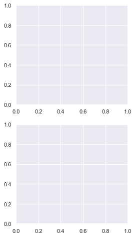
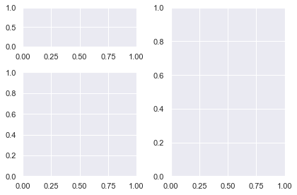
fig, axes = plt.subplots(nrows=3, ncols=1)
This creates a Figure and Subplots in a 3×1 grid. The Numpy array axes has shape (nrows, ncols) the same shape as the grid, in this case (3,) (it’s a 1D array since one of nrows or ncols is 1). Access each Subplot using Numpy slice notation and call the plot() method to plot a line graph.
Once all Subplots have been plotted, call plt.tight_layout() to ensure no parts of the plots overlap. Finally, call plt.show() to display your plot.
# Import necessary modules and (optionally) set Seaborn style
import matplotlib.pyplot as plt
import seaborn as sns; sns.set()
import numpy as np # Generate data to plot
linear = [x for x in range(5)]
square = [x**2 for x in range(5)]
cube = [x**3 for x in range(5)] # Generate Figure object and Axes object with shape 3x1
fig, axes = plt.subplots(nrows=3, ncols=1) # Access first Subplot and plot linear numbers
axes[0].plot(linear) # Access second Subplot and plot square numbers
axes[1].plot(square) # Access third Subplot and plot cube numbers
axes[2].plot(cube) plt.tight_layout()
plt.show()
Matplotlib Figures and Axes
Up until now, you have probably made all your plots with the functions in matplotlib.pyplot i.e. all the functions that start with plt..
These work nicely when you draw one plot at a time. But to draw multiple plots on one Figure, you need to learn the underlying classes in matplotlib.
Let’s look at an image that explains the main classes from the AnatomyOfMatplotlib tutorial:
To quote AnatomyOfMatplotlib:
The Figure is the top-level container in this hierarchy. It is the overall window/page that everything is drawn on. You can have multiple independent figures and Figures can contain multiple Axes.
Most plotting ocurs on an Axes. The axes is effectively the area that we plot data on and any ticks/labels/etc associated with it. Usually we’ll set up an Axes with a call to subplots (which places Axes on a regular grid), so in most cases, Axes and Subplot are synonymous.
Each Axes has an XAxis and a YAxis. These contain the ticks, tick locations, labels, etc. In this tutorial, we’ll mostly control ticks, tick labels, and data limits through other mechanisms, so we won’t touch the individual Axis part of things all that much. However, it is worth mentioning here to explain where the term Axes comes from.
The typical variable names for each object are:
Figure – fig or f,
Axes (plural) – axes or axs,
Axes (singular) – ax or a
The word Axes refers to the area you plot on and is synonymous with Subplot. However, you can have multiple Axes (Subplots) on a Figure. In speech and writing use the same word for the singular and plural form. In your code, you should make a distinction between each – you plot on a singular Axes but will store all the Axes in a Numpy array.
An Axis refers to the XAxis or YAxis – the part that gets ticks and labels.
The pyplot module implicitly works on one Figure and one Axes at a time. When we work with Subplots, we work with multiple Axes on one Figure. So, it makes sense to plot with respect to the Axes and it is much easier to keep track of everything.
The main differences between using Axes methods and pyplot are:
Always create a Figure and Axes objects on the first line
To plot, write ax.plot() instead of plt.plot().
Once you get the hang of this, you won’t want to go back to using pyplot. It’s much easier to create interesting and engaging plots this way. In fact, this is why most StackOverflow answers are written with this syntax.
All of the functions in pyplot have a corresponding method that you can call on Axes objects, so you don’t have to learn any new functions.
Let’s get to it.
Matplotlib Subplots Example
The plt.subplots() function creates a Figure and a Numpy array of Subplots/Axes objects which we store in fig and axes respectively.
Specify the number of rows and columns you want with the nrows and ncols arguments.
fig, axes = plt.subplots(nrows=3, ncols=1)
This creates a Figure and Subplots in a 3×1 grid. The Numpy array axes is the same shape as the grid, in this case (3,). Access each Subplot using Numpy slice notation and call the plot() method to plot a line graph.
Once all Subplots have been plotted, call plt.tight_layout() to ensure no parts of the plots overlap. Finally, call plt.show() to display your plot.
The most important arguments for plt.subplots() are similar to the matplotlib subplot function but can be specified with keywords. Plus, there are more powerful ones which we will discuss later.
To create a Figure with one Axes object, call it without any arguments
fig, ax = plt.subplots()
Note: this is implicitly called whenever you use the pyplot module. All ‘normal’ plots contain one Figure and one Axes.
In advanced blog posts and StackOverflow answers, you will see a line similar to this at the top of the code. It is much more Pythonic to create your plots with respect to a Figure and Axes.
To create a Grid of subplots, specify nrows and ncols – the number of rows and columns respectively
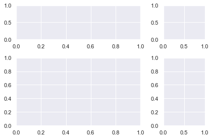
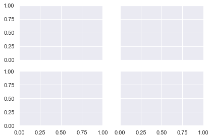
fig, axes = plt.subplots(nrows=2, ncols=2)
The variable axes is a numpy array with shape (nrows, ncols). Note that it is in the plural form to indicate it contains more than one Axes object. Another common name is axs. Choose whichever you prefer. If you call plt.subplots() without an argument name the variable ax as there is only one Axes object returned.
I will select each Axes object with slicing notation and plot using the appropriate methods. Since I am using Numpy slicing, the index of the first Axes is 0, not 1.
# Create Figure and 2x2 gris of Axes objects
fig, axes = plt.subplots(nrows=2, ncols=2) # Generate data to plot. data = np.array([1, 2, 3, 4, 5]) # Access Axes object with Numpy slicing then plot different distributions
axes[0, 0].plot(data)
axes[0, 1].plot(data**2)
axes[1, 0].plot(data**3)
axes[1, 1].plot(np.log(data)) plt.tight_layout()
plt.show()
First I import the necessary modules, then create the Figure and Axes objects using plt.subplots(). The Axes object is a Numpy array with shape (2, 2) and I access each subplot via Numpy slicing before doing a line plot of the data. Then, I call plt.tight_layout() to ensure the axis labels don’t overlap with the plots themselves. Finally, I call plt.show() as you do at the end of all matplotlib plots.
Matplotlib Subplots Title
To add an overall title to the Figure, use plt.suptitle().
To add a title to each Axes, you have two methods to choose from:
ax.set_title('bar')
ax.set(title='bar')
In general, you can set anything you want on an Axes using either of these methods. I recommend using ax.set() because you can pass any setter function to it as a keyword argument. This is faster to type, takes up fewer lines of code and is easier to read.
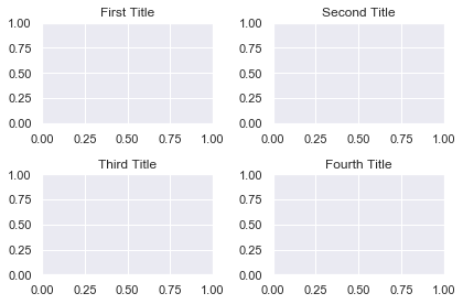
Let’s set the title, xlabel and ylabel for two Subplots using both methods for comparison
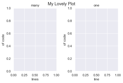
# Unpack the Axes object in one line instead of using slice notation
fig, (ax1, ax2) = plt.subplots(nrows=1, ncols=2) # First plot - 3 lines
ax1.set_title('many')
ax1.set_xlabel('lines')
ax1.set_ylabel('of code') # Second plot - 1 line
ax2.set(title='one', xlabel='line', ylabel='of code') # Overall title
plt.suptitle('My Lovely Plot')
plt.tight_layout()
plt.show()
Clearly using ax.set() is the better choice.
Note that I unpacked the Axes object into individual variables on the first line. You can do this instead of Numpy slicing if you prefer. It is easy to do with 1D arrays. Once you create grids with multiple rows and columns, it’s easier to read if you don’t unpack them.
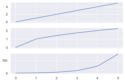
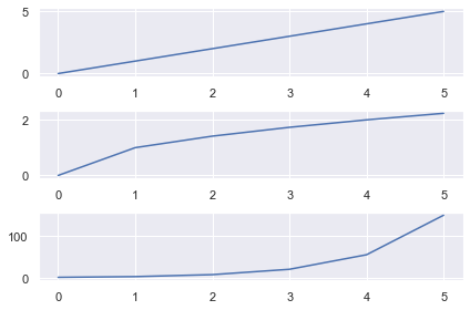
Matplotlib Subplots Share X Axis
To share the x axis for subplots in matplotlib, set sharex=True in your plt.subplots() call.
# Generate data
data = [0, 1, 2, 3, 4, 5] # 3x1 grid that shares the x axis
fig, axes = plt.subplots(nrows=3, ncols=1, sharex=True) # 3 different plots
axes[0].plot(data)
axes[1].plot(np.sqrt(data))
axes[2].plot(np.exp(data)) plt.tight_layout()
plt.show()
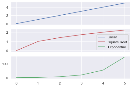
Here I created 3 line plots that show the linear, square root and exponential of the numbers 0-5.
As I used the same numbers, it makes sense to share the x-axis.
Here I wrote the same code but set sharex=False (the default behavior). Now there are unnecessary axis labels on the top 2 plots.
You can also share the y axis for plots by setting sharey=True in your plt.subplots() call.
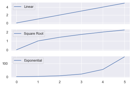
Matplotlib Subplots Legend
To add a legend to each Axes, you must
Label it using the label keyword
Call ax.legend() on the Axes you want the legend to appear
Let’s look at the same plot as above but add a legend to each Axes.
# Generate data, 3x1 plot with shared XAxis
data = [0, 1, 2, 3, 4, 5]
fig, axes = plt.subplots(nrows=3, ncols=1, sharex=True) # Plot the distributions and label each Axes
axes[0].plot(data, label='Linear')
axes[1].plot(np.sqrt(data), label='Square Root')
axes[2].plot(np.exp(data), label='Exponential') # Add a legend to each Axes with default values
for ax in axes: ax.legend() plt.tight_layout()
plt.show()
The legend now tells you which function has been applied to the data. I used a for loop to call ax.legend() on each of the Axes. I could have done it manually instead by writing:
Instead of having 3 legends, let’s just add one legend to the Figure that describes each line. Note that you need to change the color of each line, otherwise the legend will show three blue lines.
handles – the lines/plots you want to add to the legend (list)
labels – the labels you want to give each line (list)
Get the handles by storing the output of you ax.plot() calls in a list. You need to create the list of labels yourself. Then call legend() on the Axes you want to add the legend to.
# Generate data and 3x1 grid with a shared x axis
data = [0, 1, 2, 3, 4, 5]
fig, axes = plt.subplots(nrows=3, ncols=1, sharex=True) # Store the output of our plot calls to use as handles
# Plot returns a list of length 1, so unpack it using a comma
linear, = axes[0].plot(data, 'b')
sqrt, = axes[1].plot(np.sqrt(data), 'r')
exp, = axes[2].plot(np.exp(data), 'g') # Create handles and labels for the legend
handles = [linear, sqrt, exp]
labels = ['Linear', 'Square Root', 'Exponential'] # Draw legend on first Axes
axes[0].legend(handles, labels) plt.tight_layout()
plt.show()
First I generated the data and a 3×1 grid. Then I made three ax.plot() calls and applied different functions to the data.
Note that ax.plot() returns a list of matplotlib.line.Line2D objects. You have to pass these Line2D objects to ax.legend() and so need to unpack them first.
Standard unpacking syntax in Python is:
a, b = [1, 2]
# a = 1, b = 2
However, each ax.plot() call returns a list of length 1. To unpack these lists, write
x, = [5]
# x = 5
If you just wrote x = [5] then x would be a list and not the object inside the list.
After the plot() calls, I created 2 lists of handles and labels which I passed to axes[0].legend() to draw it on the first plot.
In the above plot, I changed thelegend call to axes[1].legend(handles, labels) to plot it on the second (middle) Axes.
Matplotlib Subplots Size
You have total control over the size of subplots in matplotlib.
You can either change the size of the entire Figure or the size of the Subplots themselves.
First, let’s look at changing the Figure.
Matplotlib Figure Size
If you are happy with the size of your subplots but you want the final image to be larger/smaller, change the Figure.
If you’ve read my article on the matplotlib subplot function, you know to use the plt.figure() function to to change the Figure. Fortunately, any arguments passed to plt.subplots() are also passed to plt.figure(). So, you don’t have to add any extra lines of code, just keyword arguments.
I created a 2×1 plot and set the Figure size with the figsize argument. It accepts a tuple of 2 numbers – the (width, height) of the image in inches.
So, I created a plot 3 inches wide and 6 inches long – figsize=(3, 6).
# 2x1 grid - twice as long as it is wide
fig, axes = plt.subplots(nrows=2, ncols=1, figsize=plt.figaspect(2))
plt.show()
You can set a more general Figure size with the matplotlib figaspect function. It lets you set the aspect ratio (height/width) of the Figure.
Above, I created a Figure twice as long as it is wide by setting figsize=plt.figaspect(2).
Note: Remember the aspect ratio (height/width) formula by recalling that height comes first in the alphabet before width.
Matplotlib Subplots Different Sizes
If you have used plt.subplot() before (I’ve written a whole tutorial on this too), you’ll know that the grids you create are limited. Each Subplot must be part of a regular grid i.e. of the form 1/x for some integer x. If you create a 2×1 grid, you have 2 rows and each row takes up 1/2 of the space. If you create a 3×2 grid, you have 6 subplots and each takes up 1/6 of the space.
Using plt.subplots() you can create a 2×1 plot with 2 rows that take up any fraction of space you want.
Let’s make a 2×1 plot where the top row takes up 1/3 of the space and the bottom takes up 2/3.
You do this by specifying the gridspec_kw argument and passing a dictionary of values. The main arguments we are interested in are width_ratios and height_ratios. They accept lists that specify the width ratios of columns and height ratios of the rows. In this example the top row is 1/3 of the Figure and the bottom is 2/3. Thus the height ratio is 1:2 or [1, 2] as a list.
# 2 x1 grid where top is 1/3 the size and bottom is 2/3 the size
fig, axes = plt.subplots(nrows=2, ncols=1, gridspec_kw={'height_ratios': [1, 2]}) plt.tight_layout()
plt.show()
The only difference between this and a regular 2×1 plt.subplots() call is the gridspec_kw argument. It accepts a dictionary of values. These are passed to the matplotlib GridSpec constructor (the underlying class that creates the grid).
Let’s create a 2×2 plot with the same [1, 2] height ratios but let’s make the left hand column take up 3/4 of the space.
# Heights: Top row is 1/3, bottom is 2/3 --> [1, 2]
# Widths : Left column is 3/4, right is 1/4 --> [3, 1]
ratios = {'height_ratios': [1, 2], 'width_ratios': [3, 1]} fig, axes = plt.subplots(nrows=2, ncols=2, gridspec_kw=ratios) plt.tight_layout()
plt.show()
Everything is the same as the previous plot but now we have a 2×2 grid and have specified width_ratios. Since the left column takes up 3/4 of the space and the right takes up 1/4 the ratios are [3, 1].
Matplotlib Subplots Size
In the previous examples, there were white lines that cross over each other to separate the Subplots into a clear grid. But sometimes you will not have that to guide you. To create a more complex plot, you have to manually add Subplots to the grid.
You could do this using the plt.subplot() function. But since we are focusing on Figure and Axes notation in this article, I’ll show you how to do it another way.
You need to use the fig.add_subplot() method and it has the same notation as plt.subplot(). Since it is a Figure method, you first need to create one with the plt.figure() function.
fig = plt.figure()
<Figure size 432x288 with 0 Axes>
The hardest part of creating a Figure with different sized Subplots in matplotlib is figuring out what fraction of space each Subplot takes up.
So, it’s a good idea to know what you are aiming for before you start. You could sketch it on paper or draw shapes in PowerPoint. Once you’ve done this, everything else is much easier.
I’m going to create this shape.
I’ve labeled the fraction each Subplot takes up as we need this for our fig.add_subplot() calls.
I’ll create the biggest Subplot first and the others in descending order.
The right hand side is half of the plot. It is one of two plots on a Figure with 1 row and 2 columns. To select it with fig.add_subplot(), you need to set index=2.
Remember that indexing starts from 1 for the functions plt.subplot() and fig.add_subplot().
In the image, the blue numbers are the index values each Subplot has.
ax1 = fig.add_subplot(122)
As you are working with Axes objects, you need to store the result of fig.add_subplot() so that you can plot on it afterwards.
Now, select the bottom left Subplot in a a 2×2 grid i.e. index=3
ax2 = fig.add_subplot(223)
Lastly, select the top two Subplots on the left hand side of a 4×2 grid i.e. index=1 and index=3.
# Initialise Figure
fig = plt.figure() # Add 4 Axes objects of the size we want
ax1 = fig.add_subplot(122)
ax2 = fig.add_subplot(223)
ax3 = fig.add_subplot(423)
ax4 = fig.add_subplot(421) plt.tight_layout(pad=0.1)
plt.show()
Perfect! Breaking the Subplots down into their individual parts and knowing the shape you want, makes everything easier.
Now, let’s do something you can’t do with plt.subplot(). Let’s have 2 plots on the left hand side with the bottom plot twice the height as the top plot.
Like with the above plot, the right hand side is half of a plot with 1 row and 2 columns. It is index=2.
So, the first two lines are the same as the previous plot
fig = plt.figure()
ax1 = fig.add_subplot(122)
The top left takes up 1/3 of the space of the left-hand half of the plot. Thus, it takes up 1/3 x 1/2 = 1/6 of the total plot. So, it is index=1 of a 3×2 grid.
ax2 = fig.add_subplot(321)
The final subplot takes up 2/3 of the remaining space i.e. index=3 and index=5 of a 3×2 grid. But you can’t add both of these indexes as that would add two Subplots to the Figure. You need a way to add one Subplot that spans two rows.
You need the matplotlib subplot2grid function – plt.subplot2grid(). It returns an Axes object and adds it to the current Figure.
shape – tuple of 2 integers – the shape of the overall grid e.g. (3, 2) has 3 rows and 2 columns.
loc – tuple of 2 integers – the location to place the Subplot in the grid. It uses 0-based indexing so (0, 0) is first row, first column and (1, 2) is second row, third column.
rowspan – integer, default 1- number of rows for the Subplot to span to the right
colspan – integer, default 1 – number of columns for the Subplot to span down
From those definitions, you need to select the middle left Subplot and set rowspan=2 so that it spans down 2 rows.
Thus, the arguments you need for subplot2grid are:
shape=(3, 2) – 3×2 grid
loc=(1, 0) – second row, first colunn (0-based indexing)
Sidenote: why matplotlib chose 0-based indexing for loc when everything else uses 1-based indexing is a mystery to me. One way to remember it is that loc is similar to locating. This is like slicing Numpy arrays which use 0-indexing. Also, if you use GridSpec, you will often use Numpy slicing to choose the number of rows and columns that Axes span.
If you aren’t happy with the spacing between plots that plt.tight_layout() provides, manually adjust the spacing with the matplotlib subplots_adjust function.
It takes 6 optional, self explanatory arguments. Each is a float in the range [0.0, 1.0] and is a fraction of the font size:
left, right, bottom and top is the spacing on each side of the Suplots
Now I’ve decreased the height and width between Subplots to 0.05 and there is hardly any space between them.
To avoid loads of similar examples, I recommend you play around with the arguments to get a feel for how this function works.
Matplotlib Subplots Colorbar
Adding a colorbar to each Axes is similar to adding a legend. You store the ax.plot() call in a variable and pass it to fig.colorbar().
Colorbars are Figure methods since they are placed on the Figure itself and not the Axes. Yet, they do take up space from the Axes they are placed on.
Let’s look at an example.
# Generate two 10x10 arrays of random numbers in the range [0.0, 1.0]
data1 = np.random.random((10, 10))
data2 = np.random.random((10, 10)) # Initialise Figure and Axes objects with 1 row and 2 columns
# Constrained_layout=True is better than plt.tight_layout()
# Make twice as wide as it is long with figaspect
fig, axes = plt.subplots(nrows=1, ncols=2, constrained_layout=True, figsize=plt.figaspect(1/2)) pcm1 = axes[0].pcolormesh(data1, cmap='Blues')
# Place first colorbar on first column - index 0
fig.colorbar(pcm1, ax=axes[0]) pcm2 = axes[1].pcolormesh(data2, cmap='Greens')
# Place second colorbar on second column - index 1
fig.colorbar(pcm2, ax=axes[1]) plt.show()
First, I generated two 10×10 arrays of random numbers in the range [0.0, 1.0] using the np.random.random() function. Then I initialized the 1×2 grid with plt.subplots().
The keyword argument constrained_layout=True achieves a similar result to calling plt.tight_layout(). However, tight_layout only checks for tick labels, axis labels and titles. Thus, it ignores colorbars and legends and often produces bad looking plots. Fortunately, constrained_layout takes colorbars and legends into account. Thus, it should be your go-to when automatically adjusting these types of plots.
Finally, I set figsize=plt.figaspect(1/2) to ensure the plots aren’t too squashed together.
After that, I plotted the first heatmap, colored it blue and saved it in the variable pcm1. I passed that to fig.colorbar() and placed it on the first column – axes[0] with the ax keyword argument. It’s a similar story for the second heatmap.
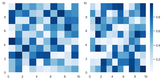
The more Axes you have, the fancier you can be with placing colorbars in matplotlib. Now, let’s look at a 2×2 example with 4 Subplots but only 2 colorbars.
# Set seed to reproduce results
np.random.seed(1) # Generate 4 samples of the same data set using a list comprehension # and assignment unpacking
data1, data2, data3, data4 = [np.random.random((10, 10)) for _ in range(4)] # 2x2 grid with constrained layout
fig, axes = plt.subplots(nrows=2, ncols=2, constrained_layout=True) # First column heatmaps with same colormap
pcm1 = axes[0, 0].pcolormesh(data1, cmap='Blues')
pcm2 = axes[1, 0].pcolormesh(data2, cmap='Blues') # First column colorbar - slicing selects all rows, first column
fig.colorbar(pcm1, ax=axes[:, 0]) # Second column heatmaps with same colormap
pcm3 = axes[0, 1].pcolormesh(data3+1, cmap='Greens')
pcm4 = axes[1, 1].pcolormesh(data4+1, cmap='Greens') # Second column colorbar - slicing selects all rows, second column
# Half the size of the first colorbar
fig.colorbar(pcm3, ax=axes[:, 1], shrink=0.5) plt.show()
If you pass a list of Axes to ax, matplotlib places the colorbar along those Axes. Moreover, you can specify where the colorbar is with the location keyword argument. It accepts the strings 'bottom', 'left', 'right', 'top' or 'center'.
The code is similar to the 1×2 plot I made above. First, I set the seed to 1 so that you can reproduce the results – you will soon plot this again with the colorbars in different places.
I used a list comprehension to generate 4 samples of the same dataset. Then I created a 2×2 grid with plt.subplots() and set constrained_layout=True to ensure nothing overlaps.
Then I made the plots for the first column – axes[0, 0] and axes[1, 0] – and saved their output. I passed one of them to fig.colorbar(). It doesn’t matter which one of pcm1 or pcm2 I pass since they are just different samples of the same dataset. I set ax=axes[:, 0] using Numpy slicing notation, that is all rows : and the first column 0.
It’s a similar process for the second column but I added 1 to data3 and data4 to give a range of numbers in [1.0, 2.0] instead. Lastly, I set shrink=0.5 to make the colorbar half its default size.
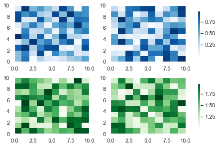
Now, let’s plot the same data with the same colors on each row rather than on each column.
# Same as above
np.random.seed(1)
data1, data2, data3, data4 = [np.random.random((10, 10)) for _ in range(4)]
fig, axes = plt.subplots(nrows=2, ncols=2, constrained_layout=True) # First row heatmaps with same colormap
pcm1 = axes[0, 0].pcolormesh(data1, cmap='Blues')
pcm2 = axes[0, 1].pcolormesh(data2, cmap='Blues') # First row colorbar - placed on first row, all columns
fig.colorbar(pcm1, ax=axes[0, :], shrink=0.8) # Second row heatmaps with same colormap
pcm3 = axes[1, 0].pcolormesh(data3+1, cmap='Greens')
pcm4 = axes[1, 1].pcolormesh(data4+1, cmap='Greens') # Second row colorbar - placed on second row, all columns
fig.colorbar(pcm3, ax=axes[1, :], shrink=0.8) plt.show()
This code is similar to the one above but the plots of the same color are on the same row rather than the same column. I also shrank the colorbars to 80% of their default size by setting shrink=0.8.
Finally, let’s set the blue colorbar to be on the bottom of the heatmaps.
You can change the location of the colorbars with the location keyword argument in fig.colorbar(). The only difference between this plot and the one above is this line
If you increase the figsize argument, this plot will look much better – at the moment it’s quite cramped.
I recommend you play around with matplotlib colorbar placement. You have total control over how many colorbars you put on the Figure, their location and how many rows and columns they span. These are some basic ideas but check out the docs to see more examples of how you can place colorbars in matplotlib.
Matplotlib Subplot Grid
I’ve spoken about GridSpec a few times in this article. It is the underlying class that specifies the geometry of the grid that a subplot can be placed in.
You can create any shape you want using plt.subplots() and plt.subplot2grid(). But some of the more complex shapes are easier to create using GridSpec. If you want to become a total pro with matplotlib, check out the docs and look out for my article discussing it in future.
Summary
You can now create any shape you can imagine in matplotlib. Congratulations! This is a huge achievement. Don’t worry if you didn’t fully understand everything the first time around. I recommend you bookmark this article and revisit it from time to time.
You’ve learned the underlying classes in matplotlib: Figure, Axes, XAxis and YAxis and how to plot with respect to them. You can write shorter, more readable code by using these methods and ax.set() to add titles, xlabels and many other things to each Axes. You can create more professional looking plots by sharing the x-axis and y-axis and add legends anywhere you like.
You can create Figures of any size that include Subplots of any size – you’re no longer restricted to those that take up 1/xth of the plot. You know that to make the best plots, you should plan ahead and figure out the shape you are aiming for.
You know when to use plt.tight_layout() (ticks, labels and titles) and constrained_layout=True (legends and colorbars) and how to manually adjust spacing between plots with plt.subplots_adjust().
Finally, you can add colorbars to as many Axes as you want and place them wherever you’d like.
You’ve done everything now. All that is left is to practice these plots so that you can quickly create amazing plots whenever you want.
Where To Go From Here?
Do you wish you could be a programmer full-time but don’t know how to start?
Check out my pure value-packed webinar where I teach you to become a Python freelancer in 60 days or your money back!
It doesn’t matter if you’re a Python novice or Python pro. If you are not making six figures/year with Python right now, you will learn something from this webinar.
These are proven, no-BS methods that get you results fast.
This webinar won’t be online forever. Click the link below before the seats fill up and learn how to become a Python freelancer, guaranteed.
This tutorial is all about the AND operator of Python’s re library. You may ask: what? (And rightly so.)
Sure, there’s the OR operator (example: 'iPhone|iPad'). But what’s the meaning of matching one regular expression AND another?
There are different interpretations for the AND operator in a regular expression (regex):
Ordered: Match one regex pattern after another. In other words, you first match pattern A AND then you match pattern B. Here the answer is simple: you use the pattern AB to match both.
Unordered: Match multiple patterns in a string but in no particular order (source). In this case, you’ll use a bag-of-words approach.
I’ll discuss both in the following. (You can also watch the video as you read the tutorial.)
Ordered Python Regex AND Operator
Given a string. Say, your goal is to find all substrings that match string 'iPhone', followed by string 'iPad'. You can view this as the AND operator of two regular expressions. How can you achieve this?
The straightforward AND operation of both strings is the regular expression pattern iPhoneiPad.
In the following example, you want to match pattern ‘aaa’ and pattern ‘bbb’—in this order.
>>> import re
>>> text = 'aaabaaaabbb'
>>> A = 'aaa'
>>> B = 'bbb'
>>> re.findall(A+B, text)
['aaabbb']
>>>
You use the re.findall() method. In case you don’t know it, here’s the definition from the Finxter blog article:
The re.findall(pattern, string) method finds all occurrences of the pattern in the string and returns a list of all matching substrings.
The first argument is the pattern A+B which evaluates to 'aaabbb'. There’s nothing fancy about this: each time you write a string consisting of more than one character, you essentially use the ordered AND operator.
The second argument is the text 'aaabaaaabbb' which you want to search for the pattern.
The result shows that there’s a matching substring in the text: 'aaabbb'.
Unordered Python Regex AND Operator
But what if you want to search a given text for pattern A AND pattern B—but in no particular order? In other words: if both patterns appear anywhere in the string, the whole string should be returned as a match.
Now this is a bit more complicated because any regular expression pattern is ordered from left to right. A simple solution is to use the lookahead assertion (?.*A) to check whether regex A appears anywhere in the string. (Note we assume a single line string as the .* pattern doesn’t match the newline character by default.)
Let’s first have a look at the minimal solution to check for two patterns anywhere in the string (say, patterns 'hi' AND 'you').
>>> import re
>>> pattern = '(?=.*hi)(?=.*you)'
>>> re.findall(pattern, 'hi how are yo?')
[]
>>> re.findall(pattern, 'hi how are you?')
['']
In the first example, both words do not appear. In the second example, they do.
But how does the lookahead assertion work? You must know that any other regex pattern “consumes” the matched substring. The consumed substring cannot be matched by any other part of the regex.
Think of the lookahead assertion as a non-consuming pattern match. The regex engine goes from the left to the right—searching for the pattern. At each point, it has one “current” position to check if this position is the first position of the remaining match. In other words, the regex engine tries to “consume” the next character as a (partial) match of the pattern.
The advantage of the lookahead expression is that it doesn’t consume anything. It just “looks ahead” starting from the current position whether what follows would theoretically match the lookahead pattern. If it doesn’t, the regex engine cannot move on.
A simple example of lookahead. The regular expression engine matches (“consumes”) the string partially. Then it checks whether the remaining pattern could be matched without actually matching it.
Let’s go back to the expression (?=.*hi)(?=.*you) to match strings that contain both 'hi' and 'you'. Why does it work?
The reason is that the lookahead expressions don’t consume anything. You first search for an arbitrary number of characters .*, followed by the word hi. But because the regex engine hasn’t consumed anything, it’s still at the same position at the beginning of the string. So, you can repeat the same for the word you.
Note that this method doesn’t care about the order of the two words:
>>> import re
>>> pattern = '(?=.*hi)(?=.*you)'
>>> re.findall(pattern, 'hi how are you?')
['']
>>> re.findall(pattern, 'you are how? hi!')
['']
No matter which word "hi" or "you" appears first in the text, the regex engine finds both.
You may ask: why’s the output the empty string? The reason is that the regex engine hasn’t consumed any character. It just checked the lookaheads. So the easy fix is to consume all characters as follows:
Now, the whole string is a match because after checking the lookahead with '(?=.*hi)(?=.*you)', you also consume the whole string '.*'.
Python Regex Not
How can you search a string for substrings that do NOT match a given pattern? In other words, what’s the “negative pattern” in Python regular expressions?
The answer is two-fold:
If you want to match all characters except a set of specific characters, you can use the negative character class [^...].
If you want to match all substrings except the ones that match a regex pattern, you can use the feature of negative lookahead(?!...).
Here’s an example for the negative character class:
>>> import re
>>> re.findall('[^a-m]', 'aaabbbaababmmmnoopmmaa')
['n', 'o', 'o', 'p']
And here’s an example for the negative lookahead pattern to match all “words that are not followed by words”:
The negative lookahead (?![a-z]+) doesn’t consume (match) any character. It just checks whether the pattern [a-z]+ does NOT match at a given position. The only times this happens is just before the empty space and the end of the string.
[Collection] What Are The Different Python Re Quantifiers?
The “and”, “or”, and “not” operators are not the only regular expression operators you need to understand. So what are other operators?
Next, you’ll get a quick and dirty overview of the most important regex operations and how to use them in Python. Here are the most important regex quantifiers:
Quantifier
Description
Example
.
The wild-card (‘dot’) matches any character in a string except the newline character ‘n’.
Regex ‘…’ matches all words with three characters such as ‘abc’, ‘cat’, and ‘dog’.
*
The zero-or-more asterisk matches an arbitrary number of occurrences (including zero occurrences) of the immediately preceding regex.
Regex ‘cat*’ matches the strings ‘ca’, ‘cat’, ‘catt’, ‘cattt’, and ‘catttttttt’.
?
The zero-or-one matches (as the name suggests) either zero or one occurrences of the immediately preceding regex.
Regex ‘cat?’ matches both strings ‘ca’ and ‘cat’ — but not ‘catt’, ‘cattt’, and ‘catttttttt’.
+
The at-least-one matches one or more occurrences of the immediately preceding regex.
Regex ‘cat+’ does not match the string ‘ca’ but matches all strings with at least one trailing character ‘t’ such as ‘cat’, ‘catt’, and ‘cattt’.
^
The start-of-string matches the beginning of a string.
Regex ‘^p’ matches the strings ‘python’ and ‘programming’ but not ‘lisp’ and ‘spying’ where the character ‘p’ does not occur at the start of the string.
$
The end-of-string matches the end of a string.
Regex ‘py$’ would match the strings ‘main.py’ and ‘pypy’ but not the strings ‘python’ and ‘pypi’.
A|B
The OR matches either the regex A or the regex B. Note that the intuition is quite different from the standard interpretation of the or operator that can also satisfy both conditions.
Regex ‘(hello)|(hi)’ matches strings ‘hello world’ and ‘hi python’. It wouldn’t make sense to try to match both of them at the same time.
AB
The AND matches first the regex A and second the regex B, in this sequence.
We’ve already seen it trivially in the regex ‘ca’ that matches first regex ‘c’ and second regex ‘a’.
Note that I gave the above operators some more meaningful names (in bold) so that you can immediately grasp the purpose of each regex. For example, the ‘^’ operator is usually denoted as the ‘caret’ operator. Those names are not descriptive so I came up with more kindergarten-like words such as the “start-of-string” operator.
We’ve already seen many examples but let’s dive into even more!
import re text = ''' Ha! let me see her: out, alas! he's cold: Her blood is settled, and her joints are stiff; Life and these lips have long been separated: Death lies on her like an untimely frost Upon the sweetest flower of all the field. ''' print(re.findall('.a!', text)) '''
Finds all occurrences of an arbitrary character that is
followed by the character sequence 'a!'.
['Ha!'] ''' print(re.findall('is.*and', text)) '''
Finds all occurrences of the word 'is',
followed by an arbitrary number of characters
and the word 'and'.
['is settled, and'] ''' print(re.findall('her:?', text)) '''
Finds all occurrences of the word 'her',
followed by zero or one occurrences of the colon ':'.
['her:', 'her', 'her'] ''' print(re.findall('her:+', text)) '''
Finds all occurrences of the word 'her',
followed by one or more occurrences of the colon ':'.
['her:'] ''' print(re.findall('^Ha.*', text)) '''
Finds all occurrences where the string starts with
the character sequence 'Ha', followed by an arbitrary
number of characters except for the new-line character. Can you figure out why Python doesn't find any?
[] ''' print(re.findall('n$', text)) '''
Finds all occurrences where the new-line character 'n'
occurs at the end of the string.
['n'] ''' print(re.findall('(Life|Death)', text)) '''
Finds all occurrences of either the word 'Life' or the
word 'Death'.
['Life', 'Death'] '''
In these examples, you’ve already seen the special symbol ‘n’ which denotes the new-line character in Python (and most other languages). There are many special characters, specifically designed for regular expressions. Next, we’ll discover the most important special symbols.
Related Re Methods
There are seven important regular expression methods which you must master:
The re.findall(pattern, string) method returns a list of string matches. Read more in our blog tutorial.
The re.search(pattern, string) method returns a match object of the first match. Read more in our blog tutorial.
The re.match(pattern, string) method returns a match object if the regex matches at the beginning of the string. Read more in our blog tutorial.
The re.fullmatch(pattern, string) method returns a match object if the regex matches the whole string. Read more in our blog tutorial.
The re.compile(pattern) method prepares the regular expression pattern—and returns a regex object which you can use multiple times in your code. Read more in our blog tutorial.
The re.split(pattern, string) method returns a list of strings by matching all occurrences of the pattern in the string and dividing the string along those. Read more in our blog tutorial.
The re.sub(The re.sub(pattern, repl, string, count=0, flags=0) method returns a new string where all occurrences of the pattern in the old string are replaced by repl. Read more in our blog tutorial.
These seven methods are 80% of what you need to know to get started with Python’s regular expression functionality.
Where to Go From Here?
You’ve learned everything you need to know about the Python Regex AND Operator.
Summary:
There are different interpretations for the AND operator in a regular expression (regex):
Ordered: Match one regex pattern after another. In other words, you first match pattern A AND then you match pattern B. Here the answer is simple: you use the pattern AB to match both.
Unordered: Match multiple patterns in a string but in no particular order. In this case, you’ll use a bag-of-words approach.
Want to earn money while you learn Python? Average Python programmers earn more than $50 per hour. You can certainly become average, can’t you?
Join the free webinar that shows you how to become a thriving coding business owner online!
The first argument is the pattern (iPhone|iPad). It either matches the first part right in front of the or symbol |—which is iPhone—or the second part after it—which is iPad.
The second argument is the text 'Buy now: iPhone only $399 with free iPad' which you want to search for the pattern.
The result shows that there are two matching substrings in the text: 'iPhone' and 'iPad'.
Python Regex Or: Examples
Let’s study some more examples to teach you all the possible uses and border cases—one after another.
You start with the previous example:
>>> import re
>>> text = 'Buy now: iPhone only $399 with free iPad'
>>> re.findall('(iPhone|iPad)', text)
['iPhone', 'iPad']
In the second example, you just skipped the parentheses using the regex pattern iPhone|iPad rather than (iPhone|iPad). But no problem–it still works and generates the exact same output!
But what happens if you leave one side of the or operation empty?
The output is not as strange as it seems. The or operator allows for empty operands—in which case it wants to match the non-empty string. If this is not possible, it matches the empty string (so everything will be a match).
The previous example also shows that it still tries to match the non-empty string if possible. But what if the trivial empty match is on the left side of the or operand?
This shows some subtleties of the regex engine. First of all, it still matches the non-empty string if possible! But more importantly, you can see that the regex engine matches from left to right. It first tries to match the left regex (which it does on every single position in the text). An empty string that’s already matched will not be considered anymore. Only then, it tries to match the regex on the right side of the or operator.
Think of it this way: the regex engine moves from the left to the right—one position at a time. It matches the empty string every single time. Then it moves over the empty string and in some cases, it can still match the non-empty string. Each match “consumes” a substring and cannot be matched anymore. But an empty string cannot be consumed. That’s why you see the first match is the empty string and the second match is the substring 'iPhone'.
How to Nest the Python Regex Or Operator?
Okay, you’re not easily satisfied, are you? Let’s try nesting the Python regex or operator |.
>>> text = 'xxx iii zzz iii ii xxx'
>>> re.findall('xxx|iii|zzz', text)
['xxx', 'iii', 'zzz', 'iii', 'xxx']
So you can use multiple or operators in a row. Of course, you can also use the grouping (parentheses) operator to nest an arbitrary complicated construct of or operations:
But this seldomly leads to clean and readable code. And it can usually avoided easily by putting a bit of thought into your regex design.
Python Regex Or: Character Class
If you only want to match a single character out of a set of characters, the character class is a much better way of doing it:
>>> import re
>>> text = 'hello world'
>>> re.findall('[abcdefghijklmnopqrstuvwxyz]+', text)
['hello', 'world']
A shorter and more concise version would be to use the range operator within character classes:
>>> re.findall('[a-z]+', text)
['hello', 'world']
The character class is enclosed in the bracket notation [ ] and it literally means “match exactly one of the symbols in the class”. Thus, it carries the same semantics as the or operator: |. However, if you try to do something on those lines…
… you’ll first write much less concise code and, second, risk of getting confused by the output. The reason is that the parenthesis is the group operator—it captures the position and substring that matches the regex. Used in the findall() method, it only returns the content of the last matched group. This turns out to be the last character of the word 'hello' and the last character of the word 'world'.
How to Match the Or Character (Vertical Line ‘|’)?
So if the character '|' stands for the or character in a given regex, the question arises how to match the vertical line symbol '|' itself?
The answer is simple: escape the or character in your regular expression using the backslash. In particular, use 'A\|B' instead of 'A|B' to match the string 'A|B' itself. Here’s an example:
Do you really understand the outputs of this code snippet? In the first example, you’re searching for either character 'A' or character 'B'. In the second example, you’re searching for the string 'A|B' (which contains the '|' character).
Python Regex And
If there’s a Python regex “or”, there must also be an “and” operator, right?
Correct! But think about it for a moment: say, you want one regex to occur alongside another regex. In other words, you want to match regex A and regex B. So what do you do? You match regex AB.
You’ve already seen many examples of the “Python regex AND” operator—but here’s another one:
>>> import re
>>> re.findall('AB', 'AAAACAACAABAAAABAAC')
['AB', 'AB']
The simple concatenation of regex A and B already performs an implicit “and operation”.
Python Regex Not
How can you search a string for substrings that do NOT match a given pattern? In other words, what’s the “negative pattern” in Python regular expressions?
The answer is two-fold:
If you want to match all characters except a set of specific characters, you can use the negative character class [^...].
If you want to match all substrings except the ones that match a regex pattern, you can use the feature of negative lookahead(?!...).
Here’s an example for the negative character class:
>>> import re
>>> re.findall('[^a-m]', 'aaabbbaababmmmnoopmmaa')
['n', 'o', 'o', 'p']
And here’s an example for the negative lookahead pattern to match all “words that are not followed by words”:
The negative lookahead (?![a-z]+) doesn’t consume (match) any character. It just checks whether the pattern [a-z]+ does NOT match at a given position. The only times this happens is just before the empty space and the end of the string.
[Collection] What Are The Different Python Re Quantifiers?
The “and”, “or”, and “not” operators are not the only regular expression operators you need to understand. So what are other operators?
Next, you’ll get a quick and dirty overview of the most important regex operations and how to use them in Python. Here are the most important regex quantifiers:
Quantifier
Description
Example
.
The wild-card (‘dot’) matches any character in a string except the newline character ‘n’.
Regex ‘…’ matches all words with three characters such as ‘abc’, ‘cat’, and ‘dog’.
*
The zero-or-more asterisk matches an arbitrary number of occurrences (including zero occurrences) of the immediately preceding regex.
Regex ‘cat*’ matches the strings ‘ca’, ‘cat’, ‘catt’, ‘cattt’, and ‘catttttttt’.
?
The zero-or-one matches (as the name suggests) either zero or one occurrences of the immediately preceding regex.
Regex ‘cat?’ matches both strings ‘ca’ and ‘cat’ — but not ‘catt’, ‘cattt’, and ‘catttttttt’.
+
The at-least-one matches one or more occurrences of the immediately preceding regex.
Regex ‘cat+’ does not match the string ‘ca’ but matches all strings with at least one trailing character ‘t’ such as ‘cat’, ‘catt’, and ‘cattt’.
^
The start-of-string matches the beginning of a string.
Regex ‘^p’ matches the strings ‘python’ and ‘programming’ but not ‘lisp’ and ‘spying’ where the character ‘p’ does not occur at the start of the string.
$
The end-of-string matches the end of a string.
Regex ‘py$’ would match the strings ‘main.py’ and ‘pypy’ but not the strings ‘python’ and ‘pypi’.
A|B
The OR matches either the regex A or the regex B. Note that the intuition is quite different from the standard interpretation of the or operator that can also satisfy both conditions.
Regex ‘(hello)|(hi)’ matches strings ‘hello world’ and ‘hi python’. It wouldn’t make sense to try to match both of them at the same time.
AB
The AND matches first the regex A and second the regex B, in this sequence.
We’ve already seen it trivially in the regex ‘ca’ that matches first regex ‘c’ and second regex ‘a’.
Note that I gave the above operators some more meaningful names (in bold) so that you can immediately grasp the purpose of each regex. For example, the ‘^’ operator is usually denoted as the ‘caret’ operator. Those names are not descriptive so I came up with more kindergarten-like words such as the “start-of-string” operator.
We’ve already seen many examples but let’s dive into even more!
import re text = ''' Ha! let me see her: out, alas! he's cold: Her blood is settled, and her joints are stiff; Life and these lips have long been separated: Death lies on her like an untimely frost Upon the sweetest flower of all the field. ''' print(re.findall('.a!', text)) '''
Finds all occurrences of an arbitrary character that is
followed by the character sequence 'a!'.
['Ha!'] ''' print(re.findall('is.*and', text)) '''
Finds all occurrences of the word 'is',
followed by an arbitrary number of characters
and the word 'and'.
['is settled, and'] ''' print(re.findall('her:?', text)) '''
Finds all occurrences of the word 'her',
followed by zero or one occurrences of the colon ':'.
['her:', 'her', 'her'] ''' print(re.findall('her:+', text)) '''
Finds all occurrences of the word 'her',
followed by one or more occurrences of the colon ':'.
['her:'] ''' print(re.findall('^Ha.*', text)) '''
Finds all occurrences where the string starts with
the character sequence 'Ha', followed by an arbitrary
number of characters except for the new-line character. Can you figure out why Python doesn't find any?
[] ''' print(re.findall('n$', text)) '''
Finds all occurrences where the new-line character 'n'
occurs at the end of the string.
['n'] ''' print(re.findall('(Life|Death)', text)) '''
Finds all occurrences of either the word 'Life' or the
word 'Death'.
['Life', 'Death'] '''
In these examples, you’ve already seen the special symbol ‘\n’ which denotes the new-line character in Python (and most other languages). There are many special characters, specifically designed for regular expressions. Next, we’ll discover the most important special symbols.
Related Re Methods
There are seven important regular expression methods which you must master:
The re.findall(pattern, string) method returns a list of string matches. Read more in our blog tutorial.
The re.search(pattern, string) method returns a match object of the first match. Read more in our blog tutorial.
The re.match(pattern, string) method returns a match object if the regex matches at the beginning of the string. Read more in our blog tutorial.
The re.fullmatch(pattern, string) method returns a match object if the regex matches the whole string. Read more in our blog tutorial.
The re.compile(pattern) method prepares the regular expression pattern—and returns a regex object which you can use multiple times in your code. Read more in our blog tutorial.
The re.split(pattern, string) method returns a list of strings by matching all occurrences of the pattern in the string and dividing the string along those. Read more in our blog tutorial.
The re.sub(The re.sub(pattern, repl, string, count=0, flags=0) method returns a new string where all occurrences of the pattern in the old string are replaced by repl. Read more in our blog tutorial.
These seven methods are 80% of what you need to know to get started with Python’s regular expression functionality.
Where to Go From Here?
You’ve learned everything you need to know about the Python Regex Or Operator.
Summary:
Given a string. Say, your goal is to find all substrings that match either the string 'iPhone' or the string 'iPad'. How can you achieve this?
The easiest way to achieve this is the Python or operator | using the regular expression pattern (iPhone|iPad).
Want to earn money while you learn Python? Average Python programmers earn more than $50 per hour. You can certainly become average, can’t you?
Join the free webinar that shows you how to become a thriving coding business owner online!
How do you know your readers’ or customers’ thoughts on your website content? How does the star rating feature help to collect customers’ opinions?
Star rating is a feature that is used across different domains in a variety of ways. For example, it is one of the key building blocks in an eCommerce website.
Star rating helps you to know how people rank your content. It not only gives rank on your content. Also, it brings more readers to your page by the gained rating.
When you build a website, if you have got scope for implementing a star rating system and you should definitely experiment with it.
Websites use a variety of ways to allow users to rate content. For example, star rating, up-down rating, emoji rating and more.
We have seen so many examples for star rating, emoji rating and more. I grouped all those in this one single example.
I supported three UI alternatives for the rating section. Those are,
Five-star rating
Favorite rating
Emoji rating
I created a directive in PHP to configure the template for the rating appearance.
Existing plugins to implement a dynamic star rating
There are various plugins available in the market to enable star rating. The ready-made plugins are with enormous features.
For example, Rateit is a jQuery based star rating plugin. It allows embedding a star rating with a list, select and more HTML markup. It supports Font Awesome, Material icons to display rating icons.
The UpvoteJS is a JavaScript package to render a StackExchange-like rating widget.
If you are having a WordPress website, there are built-in rating plugins available. Wp-PostRatings is a popular plugin to implement rating.
Advantages of creating a custom star rating script
With a custom star rating, we can simplify the code logic instead of stuffing a lot.
And thereby, it will make it easy at the time of enhancement or maintenance phase.
It rectifies your overload with a feature-packed built-in. Also, it reduces your effort on managing a thousand lines of code for this simple UI feature.
Various types of rating options
Websites use a different type of rating options to get user’s reviews. The following list shows some of the types.
Single or multiple star rating
Facebook-like emoji rating
Simple up-down voting.
Like-unlike rating
Bar rating
The types are veries in user’s mindset while rating. For example, the like-unlike and up-down rating expects binary options 0 or 1 from the user. But with the bar rating, it can have a range of points out of some limit.
Star rating example with AJAX
I have created an AJAX-based star rating example code with PHP and jQuery.
This code will show a list of courses with an option to rate each course. The courses are from the database.
The rating element in the UI is configurable. I provided three UI alternatives for the rating section. Star, favorite and emoji ratings are there to collect users’ reviews.
While adding the rating, the code sends it to the PHP via AJAX. Then, it saves the ratings in the MySQL database.
Once rated, the user cannot rerate a course again to avoid duplicate ratings.
The following figure shows the file strucuture of the example code.
The rating example database
This section shows the structure and the SQL of the database used in this example.
I have created two tables tbl_courses and tbl_course_rating. The tbl_cources database table contains courses on which the user will add ratings.
The tbl_cource_rating table has the mapping with the tbl_cource database. It has a unique rating without duplicates.
The below script shows the CREATE statement and the data dump for these two tables. By importing this script, you can setup this example in the local environment.
sql/db_rating.sql
--
-- Database: `db_rating`
-- -- -------------------------------------------------------- --
-- Table structure for table `tbl_course`
-- CREATE TABLE `tbl_course` ( `id` int(11) NOT NULL, `name` varchar(255) NOT NULL, `description` varchar(255) NOT NULL, `period` varchar(255) NOT NULL, `availabe_seats` int(11) NOT NULL, `last_date_to_register` date NOT NULL
) ENGINE=InnoDB DEFAULT CHARSET=latin1; --
-- Dumping data for table `tbl_course`
-- INSERT INTO `tbl_course` (`id`, `name`, `description`, `period`, `availabe_seats`, `last_date_to_register`) VALUES
(1, 'Professional Training for Finantial Analyst\r\n', 'Professional Training for Finantial Analyst', '30 days', 2, '2020-01-31'),
(2, 'Enterprise Programming in Artificial Intelligence\r\n', 'Enterprise Programming in Artificial Intelligence', '30 days', 2, '2020-01-24'); -- -------------------------------------------------------- --
-- Table structure for table `tbl_course_rating`
-- CREATE TABLE `tbl_course_rating` ( `id` int(11) NOT NULL, `course_id` int(11) NOT NULL, `member_id` int(11) NOT NULL, `rating` int(11) NOT NULL
) ENGINE=InnoDB DEFAULT CHARSET=latin1; --
-- Indexes for dumped tables
-- --
-- Indexes for table `tbl_course`
--
ALTER TABLE `tbl_course` ADD PRIMARY KEY (`id`); --
-- Indexes for table `tbl_course_rating`
--
ALTER TABLE `tbl_course_rating` ADD PRIMARY KEY (`id`); --
-- AUTO_INCREMENT for dumped tables
-- --
-- AUTO_INCREMENT for table `tbl_course`
--
ALTER TABLE `tbl_course` MODIFY `id` int(11) NOT NULL AUTO_INCREMENT, AUTO_INCREMENT=3; --
-- AUTO_INCREMENT for table `tbl_course_rating`
--
ALTER TABLE `tbl_course_rating` MODIFY `id` int(11) NOT NULL AUTO_INCREMENT, AUTO_INCREMENT=95;
COMMIT;
UI design to render star rating option
In a landing page, it shows the list of courses from the database. The HTML code for this page is below.
It loads the rating element based on the PHP constant defined in a common configuration file.
The rating element will show clickable 5-stars or favorite-icons or emoji icons.
On clicking the rating element, it invokes a jQuery script to send AJAX requests to save ratings.
I created separate template files to have different types of rating UI. Those are star-rating-view.php, favorite-rating-view.php and emoji_rating_view.php.
The template files show the onClick event handling specification in the markup.
In the emoji rating template, it shows a range of five emotion icons from very-sad to very-happy.
If you are providing support on the user’s queries, you can use the emoji rating. Embedding the emoji rating will give the customer’s emotional feel on your support.
This file contains jQuery functions to prepare AJAX requests to save user ratings.
It also handles the mouse hover events to highlight the rating element. The mouseOverRating() function highlights the star or other rating elements on hovering.
Similarly, mouseOutRating() resets the rating UI back to its original form on mouse out.
The AJAX code in the addRating() prepares the request with PHP endpoint URL and data params.
It receives the server response in the AJAX success callback at which it updates the UI accordingly.
assets/js/rating.js
function mouseOverRating(courseId, rating, appearance) { if (appearance == "star") { for (var i = 1; i <= rating; i++) { $('#' + courseId + "_" + i + ' img').attr('src', "./img/" + appearance + "-filled.png"); } } else { ratingIconPrefix = "./img/" + appearance; for (var i = 1; i <= rating; i++) { if (appearance == "emoji") { ratingIconPrefix = "./img/" + appearance + "1"; } if (i == rating) { $('#' + courseId + "_" + i + ' img').attr('src', ratingIconPrefix + "-filled.png"); } } } } function mouseOutRating(courseId, userRating, appearance) { var ratingId; if (appearance == "star") { if (userRating != 0) { for (var i = 1; i <= userRating; i++) { $('#' + courseId + "_" + i + ' img').attr('src', "./img/" + appearance + "-filled.png"); } } if (userRating <= 5) { for (var i = (userRating + 1); i <= 5; i++) { $('#' + courseId + "_" + i + ' img').attr('src', "./img/" + appearance + "-open.png"); } } $(".selected img").attr('src', "./img/" + appearance + "-filled.png"); } else { ratingIconPrefix = "./img/" + appearance; if (userRating <= 5) { for (var i = 1; i <= 5; i++) { if (appearance == "emoji") { ratingIconPrefix = "./img/" + appearance + i; } if (userRating == i) { $('#' + courseId + "_" + i + ' img').attr('src', ratingIconPrefix + "-filled.png"); } else { $('#' + courseId + "_" + i + ' img').attr('src', ratingIconPrefix + "-open.png"); } } } var selectedImageSource = $(".selected img").attr('src'); if (selectedImageSource) { selectedImageSource = selectedImageSource.replace('open', "filled"); $(".selected img").attr('src', selectedImageSource); } } } function addRating(currentElement, courseId, ratingValue, appearance) { var loaderIcon = $(currentElement).closest(".row-item"); $.ajax({ url : "ajax-end-point/insertRating.php", data : "index=" + ratingValue + "&course_id=" + courseId, type : "POST", beforeSend : function() { $(loaderIcon).find("#loader-icon").show(); }, success : function(data) { loaderIcon = $(currentElement).closest(".row-item"); $(loaderIcon).find("#loader-icon").hide(); if (data != "") { $('#response-' + courseId).text(data); return false; } if (appearance == 'star') { $('#list-' + courseId + ' li').each( function(index) { $(this).addClass('selected'); if (index == $('#list-' + courseId + ' li').index( currentElement)) { return false; } }); } else { $(currentElement).addClass('selected'); } } }); }
Storing user rating to MySQL database from PHP
When the AJAX script called, it prepares a request to the PHP. In PHP, it receives the chosen rating post data and stores it in the rating database.
Though the UI displays different elements, the rating value ranges from 1 to 5. In the database, it has the mapping between the rating value, course id and member id.
The below configuration is for setting the rating element appearance. The possible values are there with a comment statement.
Common/Config.php
<?php
namespace Phppot; class Config
{ // Possible values: star | favourite | emoji const RATING_APPEARANCE = "favourite";
}
Before insert, it checks if the user added a rating already for that particular course. If so, then the code will not allow the user to rate again.
ajax-end-point/insertRating.php
<?php
namespace Phppot; use Phppot\Rating;
require_once __DIR__ . "./../Model/Rating.php";
$rating = new Rating();
// Here the user id is harcoded.
// You can integrate your authentication code here to get the logged in user id
$userId = 5; if (isset($_POST["index"], $_POST["course_id"])) { $courseId = $_POST["course_id"]; $ratingIndex = $_POST["index"]; $rowCount = $rating->isUserRatingExist($userId, $courseId); if ($rowCount == 0) { $insertId = $rating->addRating($userId, $courseId, $ratingIndex); if (empty($insertId)) { echo "Problem in adding ratings."; } } else { echo "You have added rating already."; }
}
This file displays the courses list with the rating option in a landing page.
getRatingData.php
<?php
namespace Phppot; use Phppot\Rating;
require_once "./Common/Config.php";
$config = new Config();
require_once "./Model/Rating.php";
$rating = new Rating();
// Here the user id is harcoded.
// You can integrate your authentication code here to get the logged in user id
$userId = 5; $apperance = $config::RATING_APPEARANCE; $courseResult = $rating->getCourse();
if (! empty($courseResult)) { foreach ($courseResult as $row) { $userRating = $rating->getUserRating($userId, $row['id']); $totalRating = $rating->getTotalRating($row['id']); $date = date_create($row["last_date_to_register"]); ?>
<div class="row-item"> <div class="row-title"><?php echo $row['name']; ?></div> <ul class="list-inline" id="list-<?php echo $row['id']; ?>"> <?php require $apperance . "-rating-view.php"; ?> <img src="img/loader.gif" class="loader-icon" id="loader-icon"> </ul> <div class="response" id="response-<?php echo $row['id']; ?>"></div> <p class="review-note">Total Reviews: <?php echo $totalRating; ?></p> <p class="text-address"> <label class="course-detail">Period: <?php echo $row["period"]; ?></label><label class="course-detail">Available seats: <?php echo $row["availabe_seats"]; ?></label><label class="course-detail">Last Date to Register: <?php echo date_format($date, "d M Y"); ?></label> </p>
</div>
<?php }
}
?>
In the above two PHP files, I have harcoded the user id with a PHP variable $userId. You can plugin user authentication code and get the logged-in user id.
The Rating.php is a PHP model class created for performing the rating actions.
It has functions to read courses and user ratings on them. The getUserRating() and getTotalRating() functions returns data to display the rating statistics.
The isUserRatingExist() checks the uniqueness of the user rating on a particular course.
I used prepared statements with MySQLi for executing the database queries. The source contains a generic DAO class DataSource.php for executing database operations.
Model/Rating.php
<?php
namespace Phppot; use Phppot\DataSource; class Rating
{ private $ds; function __construct() { require_once __DIR__ . './../lib/DataSource.php'; $this->ds = new DataSource(); } function getCourse() { $query = "SELECT * FROM tbl_course ORDER BY id DESC"; $result = $this->ds->select($query); return $result; } function getUserRating($userId, $courseId) { $average = 0; $avgQuery = "SELECT rating FROM tbl_course_rating WHERE member_id = ? and course_id = ?"; $paramType = 'ii'; $paramValue = array( $userId, $courseId ); $result = $this->ds->select($avgQuery, $paramType, $paramValue); if ($result > 0) { foreach ($result as $row) { $average = round($row["rating"]); } // endForeach } // endIf return $average; } function getTotalRating($courseId) { $totalVotesQuery = "SELECT * FROM tbl_course_rating WHERE course_id = ?"; $paramType = 'i'; $paramValue = array( $courseId ); $result = $this->ds->getRecordCount($totalVotesQuery, $paramType, $paramValue); return $result; } function isUserRatingExist($userId, $courseId) { $checkIfExistQuery = "select * from tbl_course_rating where member_id = ? and course_id = ?"; $userId; $courseId; $paramType = 'ii'; $paramValue = array( $userId, $courseId ); $rowCount = $this->ds->getRecordCount($checkIfExistQuery, $paramType, $paramValue); return $rowCount; } function addRating($userId, $courseId, $rating) { $insertQuery = "INSERT INTO tbl_course_rating(member_id,course_id, rating) VALUES (?,?,?) "; $paramType = 'iii'; $paramValue = array( $userId, $courseId, $rating ); $insertId = $this->ds->insert($insertQuery, $paramType, $paramValue); return $insertId; }
}
Output screenshot of different rating options with star, favorite, emoji
In the following screenshot, it displays a text in red. It is an error message to notify the user if he tries to add rating again.
Conclusion
We have seen the importance of implementing a rating script in an application. Also, we have seen the types of ratings generally used by the applications.
By supporting 3 types of rating UI components in an example script, I sure it helps you to have options. You can choose and fix one among them on a need basis.
For example, if you manage more applications, then integrate this one in all. The rating configuration allows setting based on the nature of the application.
There is no limit. We can enhance this component by adding more rating options like-unlike, up-down voting, rating with a ranger and more.
Asset allocation is the process of dividing your portfolio into stocks, bonds, and cash. A famous 1990 study by Kaplan and Ibbotson proves that asset allocation is the most important investment decision for your investment success—far more important than selecting individual securities within the broader asset classes stocks, bonds, and cash.
But what’s the best asset allocation for you?
20% stocks, 50% bonds, 30% cash
50% stocks, 50% bonds
80% stocks, 10% bonds, 10% cash
100% stocks
These different asset allocations have a significant impact on your portfolio risk and return. You must invest most of your time and effort in getting the numbers right.
This is where online tools for asset allocation come into play. They allow you to play with the numbers and see for yourself, based on historical asset class returns, what’s the most sensible investment decision for you.
The best tool for asset allocation comes from my student Ann who just started out with Python and the Python visualization framework Dash. With Python, Dash, and Flask, she has built an incredibly useful tool to help you, as an individual investor, save thousands of dollars of fees paid to investment advisors. And the best thing: it’s 100% free! Check it out.
This article is all about the start of line ^ and end of line $ regular expressions in Python’s re library. These two regexes are fundamental to all regular expressions—even outside the Python world. So invest 5 minutes now and master them once and for all!
Python Re Start-of-String (^) Regex
You can use the caret operator ^ to match the beginning of the string. For example, this is useful if you want to ensure that a pattern appears at the beginning of a string. Here’s an example:
>>> import re
>>> re.findall('^PYTHON', 'PYTHON is fun.')
['PYTHON']
The findall(pattern, string) method finds all occurrences of the pattern in the string. The caret at the beginning of the pattern ‘^PYTHON’ ensures that you match the word Python only at the beginning of the string. In the previous example, this doesn’t make any difference. But in the next example, it does:
>>> re.findall('^PYTHON', 'PYTHON! PYTHON is fun')
['PYTHON']
Although there are two occurrences of the substring ‘PYTHON’, there’s only one matching substring—at the beginning of the string.
But what if you want to match not only at the beginning of the string but at the beginning of each line in a multi-line string? In other words:
Python Re Start-of-Line (^) Regex
The caret operator, per default, only applies to the start of a string. So if you’ve got a multi-line string—for example, when reading a text file—it will still only match once: at the beginning of the string.
However, you may want to match at the beginning of each line. For example, you may want to find all lines that start with ‘Python’ in a given string.
You can specify that the caret operator matches the beginning of each line via the re.MULTILINE flag. Here’s an example showing both usages—without and with setting the re.MULTILINE flag:
>>> import re
>>> text = '''
Python is great.
Python is the fastest growing
major programming language in
the world.
Pythonistas thrive.'''
>>> re.findall('^Python', text)
[]
>>> re.findall('^Python', text, re.MULTILINE)
['Python', 'Python', 'Python']
>>>
The first output is the empty list because the string ‘Python’ does not appear at the beginning of the string.
The second output is the list of three matching substrings because the string ‘Python’ appears three times at the beginning of a line.
Python re.sub()
The re.sub(pattern, repl, string, count=0, flags=0) method returns a new string where all occurrences of the pattern in the old string are replaced by repl. Read more in the Finxter blog tutorial.
You can use the caret operator to substitute wherever some pattern appears at the beginning of the string:
>>> import re
>>> re.sub('^Python', 'Code', 'Python is \nPython') 'Code is \nPython'
Only the beginning of the string matches the regex pattern so you’ve got only one substitution.
Again, you can use the re.MULTILINE flag to match the beginning of each line with the caret operator:
>>> re.sub('^Python', 'Code', 'Python is \nPython', flags=re.MULTILINE) 'Code is \nCode'
Now, you replace both appearances of the string ‘Python’.
Python re.match(), re.search(), re.findall(), and re.fullmatch()
Let’s quickly recap the most important regex methods in Python:
The re.findall(pattern, string, flags=0) method returns a list of string matches. Read more in our blog tutorial.
The re.search(pattern, string, flags=0) method returns a match object of the first match. Read more in our blog tutorial.
The re.match(pattern, string, flags=0) method returns a match object if the regex matches at the beginning of the string. Read more in our blog tutorial.
The re.fullmatch(pattern, string, flags=0) method returns a match object if the regex matches the whole string. Read more in our blog tutorial.
You can see that all four methods search for a pattern in a given string. You can use the caret operator ^ within each pattern to match the beginning of the string. Here’s one example per method:
So you can use the caret operator to match at the beginning of the string. However, you should note that it doesn’t make a lot of sense to use it for the match() and fullmatch() methods as they, by definition, start by trying to match the first character of the string.
You can also use the re.MULTILINE flag to match the beginning of each line (rather than only the beginning of the string):
Again, it’s questionable whether this makes sense for the re.match() and re.fullmatch() methods as they only look for a match at the beginning of the string.
Python Re End of String ($) Regex
Similarly, you can use the dollar-sign operator $ to match the end of the string. Here’s an example:
>>> import re
>>> re.findall('fun$', 'PYTHON is fun')
['fun']
The findall() method finds all occurrences of the pattern in the string—although the trailing dollar-sign $ ensures that the regex matches only at the end of the string.
This can significantly alter the meaning of your regex as you can see in the next example:
>>> re.findall('fun$', 'fun fun fun')
['fun']
Although, there are three occurrences of the substring ‘fun’, there’s only one matching substring—at the end of the string.
But what if you want to match not only at the end of the string but at the end of each line in a multi-line string?
Python Re End of Line ($)
The dollar-sign operator, per default, only applies to the end of a string. So if you’ve got a multi-line string—for example, when reading a text file—it will still only match once: at the end of the string.
However, you may want to match at the end of each line. For example, you may want to find all lines that end with ‘.py’.
To achieve this, you can specify that the dollar-sign operator matches the end of each line via the re.MULTILINE flag. Here’s an example showing both usages—without and with setting the re.MULTILINE flag:
>>> import re
>>> text = '''
Coding is fun
Python is fun
Games are fun
Agreed?'''
>>> re.findall('fun$', text)
[]
>>> re.findall('fun$', text, flags=re.MULTILINE)
['fun', 'fun', 'fun']
>>>
The first output is the empty list because the string ‘fun’ does not appear at the end of the string.
The second output is the list of three matching substrings because the string ‘fun’ appears three times at the end of a line.
Python re.sub()
The re.sub(pattern, repl, string, count=0, flags=0) method returns a new string where all occurrences of the pattern in the old string are replaced by repl. Read more in the Finxter blog tutorial.
You can use the dollar-sign operator to substitute wherever some pattern appears at the end of the string:
>>> import re
>>> re.sub('Python$', 'Code', 'Is Python\nPython') 'Is Python\nCode'
Only the end of the string matches the regex pattern so there’s only one substitution.
Again, you can use the re.MULTILINE flag to match the end of each line with the dollar-sign operator:
Now, you replace both appearances of the string ‘Python’.
Python re.match(), re.search(), re.findall(), and re.fullmatch()
All four methods—re.findall(), re.search(), re.match(), and re.fullmatch()—search for a pattern in a given string. You can use the dollar-sign operator $ within each pattern to match the end of the string. Here’s one example per method:
>>> import re
>>> text = 'Python is Python'
>>> re.findall('Python$', text)
['Python']
>>> re.search('Python$', text)
<re.Match object; span=(10, 16), match='Python'>
>>> re.match('Python$', text)
>>> re.fullmatch('Python$', text)
>>>
So you can use the dollar-sign operator to match at the end of the string. However, you should note that it doesn’t make a lot of sense to use it for the fullmatch() methods as it, by definition, already requires that the last character of the string is part of the matching substring.
You can also use the re.MULTILINE flag to match the end of each line (rather than only the end of the whole string):
As the pattern doesn’t match the string prefix, both re.match() and re.fullmatch() return empty results.
How to Match the Caret (^) or Dollar ($) Symbols in Your Regex?
You know that the caret and dollar symbols have a special meaning in Python’s regular expression module: they match the beginning or end of each string/line. But what if you search for the caret (^) or dollar ($) symbols themselves? How can you match them in a string?
The answer is simple: escape the caret or dollar symbols in your regular expression using the backslash. In particular, use ‘\^’ instead of ‘^’ and ‘\$’ instead of ‘$’. Here’s an example:
>>> import re
>>> text = 'The product ^^^ costs $3 today.'
>>> re.findall('\^', text)
['^', '^', '^']
>>> re.findall('\$', text)
['$']
By escaping the special symbols ^ and $, you tell the regex engine to ignore their special meaning.
Where to Go From Here?
You’ve learned everything you need to know about the caret operator ^ and the dollar-sign operator $ in this regex tutorial.
Summary: The caret operator ^ matches at the beginning of a string. The dollar-sign operator $ matches at the end of a string. If you want to match at the beginning or end of each line in a multi-line string, you can set the re.MULTILINE flag in all the relevant re methods.
Want to earn money while you learn Python? Average Python programmers earn more than $50 per hour. You can become average, can’t you?
Join the free webinar that shows you how to become a thriving coding business owner online!