[20-SEC SUMMARY] Given a list of list stored in variable lst.
- To flatten a list of lists, use the list comprehension statement
[x for l in lst for x in l]. - To modify all elements in a list of lists (e.g., increment them by one), use a list comprehension of list comprehensions
[[x+1 for x in l] for l in lst].
List comprehension is a compact way of creating lists. The simple formula is [ expression + context ].
- Expression: What to do with each list element?
- Context: What list elements to select? It consists of an arbitrary number of for and if statements.
The example [x for x in range(3)] creates the list [0, 1, 2].
In this tutorial, you’ll learn three ways how to apply list comprehension to a list of lists:
- to flatten a list of lists
- to create a list of lists
- to iterate over a list of lists
Additionally, you’ll learn how to apply nested list comprehension. So let’s get started!
Python List Comprehension Flatten List of Lists
Problem: Given a list of lists. How to flatten the list of lists by getting rid of the inner lists—and keeping their elements?
Example: You want to transform a given list into a flat list like here:
lst = [[2, 2], [4], [1, 2, 3, 4], [1, 2, 3]] # ... Flatten the list here ... print(lst)
# [2, 2, 4, 1, 2, 3, 4, 1, 2, 3]
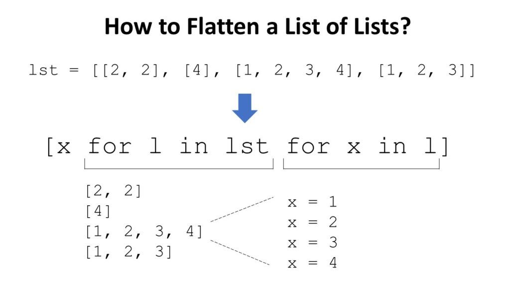
Solution: Use a nested list comprehension statement [x for l in lst for x in l] to flatten the list.
lst = [[2, 2], [4], [1, 2, 3, 4], [1, 2, 3]] # ... Flatten the list here ...
lst = [x for l in lst for x in l] print(lst)
# [2, 2, 4, 1, 2, 3, 4, 1, 2, 3]
Explanation: In the nested list comprehension statement [x for l in lst for x in l], you first iterate over all lists in the list of lists (for l in lst). Then, you iterate over all elements in the current list (for x in l). This element, you just place in the outer list, unchanged, by using it in the “expression” part of the list comprehension statement [x for l in lst for x in l].
Try It Yourself: You can execute this code snippet yourself in our interactive Python shell. Just click “Run” and test the output of this code.
Can you flatten a three-dimensional list (= a list of lists of lists)? Try it in the shell!
Python List Comprehension Create List of Lists
Problem: How to create a list of lists by modifying each element of an original list of lists?
Example: You’re given the list
[[1, 2, 3], [4, 5, 6], [7, 8, 9]]
You want to add one to each element and create a new list of lists:
[[2, 3, 4], [5, 6, 7], [8, 9, 10]]
Solution: Use two nested list comprehension statements, one to create the outer list of lists, and one to create the inner lists.
lst = [[1, 2, 3], [4, 5, 6], [7, 8, 9]]
new = [[x+1 for x in l] for l in lst]
print(new)
# [[2, 3, 4], [5, 6, 7], [8, 9, 10]]
Explanation: You’ll study more examples of two nested list comprehension statements later. The main idea is to use as “expression” of the outer list comprehension statement a list comprehension statement by itself. Remember, you can create any object you want in the expression part of your list comprehension statement.
Explore the code: You can play with the code in the interactive Python tutor that visualizes the execution step-by-step. Just click the “Next” button repeatedly to see what happens in each step of the code.
Let’s explore the third question: how to use list comprehension to iterate over a list of lists?
Python List Comprehension Over List of Lists
You’ve seen this in the previous example where you not only created a list of lists, you also iterated over each element in the list of lists. To summarize, you can iterate over a list of lists by using the statement [[modify(x) for x in l] for l in lst] using any statement or function modify(x) that returns an arbitrary object.
How Does Nested List Comprehension Work in Python?
After publishing the first version of this tutorial, many readers asked me to write a follow-up tutorial on nested list comprehension in Python. There are two interpretations of nested list comprehension:
- Coming from a computer science background, I was assuming that “nested list comprehension” refers to the creation of a list of lists. In other words: How to create a nested list with list comprehension?
- But after a bit of research, I learned that there is a second interpretation of nested list comprehension: How to use a nested for loop in the list comprehension?
How to create a nested list with list comprehension?
It is possible to create a nested list with list comprehension in Python. What is a nested list? It’s a list of lists. Here is an example:
## Nested List Comprehension
lst = [[x for x in range(5)] for y in range(3)]
print(lst)
# [[0, 1, 2, 3, 4], [0, 1, 2, 3, 4], [0, 1, 2, 3, 4]]
As you can see, we create a list with three elements. Each list element is a list by itself.
Everything becomes clear when we go back to our magic formula of list comprehension: [expression + context]. The expression part generates a new list consisting of 5 integers. The context part repeats this three times. Hence, each of the three nested lists has five elements.
If you are an advanced programmer (test your skills on the Finxter app), you may ask whether there is some aliasing going on here. Aliasing in this context means that the three list elements point to the same list [0, 1, 2, 3, 4]. This is not the case because each expression is evaluated separately, a new list is created for each of the three context executions. This is nicely demonstrated in this code snippet:
l[0].append(5)
print(l)
# [[0, 1, 2, 3, 4, 5], [0, 1, 2, 3, 4], [0, 1, 2, 3, 4]]
# ... and not [[0, 1, 2, 3, 4, 5], [0, 1, 2, 3, 4, 5], [0, 1, 2, 3, 4, 5]]
How to use a nested for loop in the list comprehension?
To be frank, the latter one is super-simple stuff. Do you remember the formula of list comprehension (= ‘[‘ + expression + context + ‘]’)?
The context is an arbitrary complex restriction construct of for loops and if restrictions with the goal of specifying the data items on which the expression should be applied.
In the expression, you can use any variable you define within a for loop in the context. Let’s have a look at an example.
Suppose you want to use list comprehension to make this code more concise (for example, you want to find all possible pairs of users in your social network application):
# BEFORE
users = ["John", "Alice", "Ann", "Zach"]
pairs = []
for x in users: for y in users: if x != y: pairs.append((x,y))
print(pairs)
#[('John', 'Alice'), ('John', 'Ann'), ('John', 'Zach'), ('Alice', 'John'), ('Alice', 'Ann'), ('Alice', 'Zach'), ('Ann', 'John'), ('Ann', 'Alice'), ('Ann', 'Zach'), ('Zach', 'John'), ('Zach', 'Alice'), ('Zach', 'Ann')]
Now, this code is a mess! How can we fix it? Simply use nested list comprehension!
# AFTER
pairs = [(x,y) for x in users for y in users if x!=y]
print(pairs)
# [('John', 'Alice'), ('John', 'Ann'), ('John', 'Zach'), ('Alice', 'John'), ('Alice', 'Ann'), ('Alice', 'Zach'), ('Ann', 'John'), ('Ann', 'Alice'), ('Ann', 'Zach'), ('Zach', 'John'), ('Zach', 'Alice'), ('Zach', 'Ann')]
As you can see, we are doing exactly the same thing as with un-nested list comprehension. The only difference is to write the two for loops and the if statement in a single line within the list notation [].
Where to Go From Here?
Enough theory, let’s get some practice!
To become successful in coding, you need to get out there and solve real problems for real people. That’s how you can become a six-figure earner easily. And that’s how you polish the skills you really need in practice. After all, what’s the use of learning theory that nobody ever needs?
Practice projects is how you sharpen your saw in coding!
Do you want to become a code master by focusing on practical code projects that actually earn you money and solve problems for people?
Then become a Python freelance developer! It’s the best way of approaching the task of improving your Python skills—even if you are a complete beginner.
Join my free webinar “How to Build Your High-Income Skill Python” and watch how I grew my coding business online and how you can, too—from the comfort of your own home.