Python is one of the most powerful and versatile programming languages available today. It is used in multiple fields, including web development, data science, artificial intelligence, and more.
As a result, Python practitioners need to have a broad range of skills to be successful. Here, we will discuss the top 10 skills to learn as a Python practitioner.
Note that I focused only on coding-related skills, not on soft skills such as communication or “agile software development“. These are vital but not part of this article.
Skill #1: Object-Oriented Programming (OOP)
Object-Oriented Programming (OOP) is a programming paradigm that uses objects and classes to organize and manage code.
OOP is a fundamental skill for Python practitioners, as it allows for the creation of efficient, robust, and reusable code. To be an effective Python programmer, you must understand the principles of OOP and be able to apply them in your code.
Data Structures and Algorithms are essential for any programmer. Data Structures are collections of data that are organized in a specific way, such as an array or linked list. Algorithms are sets of instructions used to solve specific problems. Knowing how to work with and optimize data structures and algorithms are essential for any Python practitioner.
Web Development is the process of building, creating, and maintaining websites and web applications. Python is a popular choice for web development, as it is relatively easy to learn and offers a wide range of tools and frameworks. Developing web applications with Python is a must-have skill for Python practitioners.
Machine Learning (ML) is a subset of Artificial Intelligence (AI) that enables machines to learn from data and make predictions. Python has become the go-to language for ML due to its rich and powerful libraries. To be successful in ML, Python practitioners must understand the fundamentals of ML and be able to work with ML libraries and frameworks.
Data Analysis is the process of gathering, cleaning, and interpreting data to generate insights and inform decisions. Python is an excellent language for data analysis due to its powerful libraries and tools. Knowing how to work with data in Python is an essential skill for any Python practitioner.
Automation is the process of using programming to automate mundane or repetitive tasks. Python is a popular choice for automation due to its easy-to-learn syntax and powerful libraries. Knowing how to use Python for automation can save time and allow for more efficient workflows.
Specific subskills to master:
Bash
Ansible
Puppet
Chef
Skill #7: GUI Development
GUI Development is the process of creating graphical user interfaces (GUIs) for applications. Python offers a wide range of GUI development frameworks and libraries, making it an excellent choice for GUI development. To be successful in GUI development, Python practitioners must know how to work with GUI frameworks and libraries.
Specific subskills to master:
Tkinter
PyQt
PyGTK
wxPython
PyGUI
Skill #8: Web Scraping
Web Scraping is the process of extracting data from websites. Python is an excellent language for web scraping due to its powerful libraries and tools. Knowing how to scrape websites using Python is an essential skill for any Python practitioner.
Scripting is the process of writing scripts to automate mundane or repetitive tasks. Python is a popular language for scripting due to its easy-to-learn syntax and powerful libraries. Knowing how to script in Python can save time and allow for more efficient workflows.
Data Visualization is the process of creating visual representations of data. Python offers a wide range of data visualization libraries and tools, making it an excellent choice for data visualization. Knowing how to create effective visualizations with Python is an essential skill for any Python practitioner.
Further Learning: For a complete guide on how to build your beautiful dashboard app in pure Python, check out our best-selling book Python Dash with San Francisco Based publisher NoStarch.
Conclusion
In conclusion, the top 10 skills to learn as a Python practitioner are object-oriented programming, data structures and algorithms, web development, machine learning, data analysis, automation, GUI development, web scraping, scripting, and data visualization.
Each of these skills is essential for success as a Python practitioner and can help you create powerful and efficient applications.
Highlights: retrieving user credentials from a Mongo DB, privilege escalation by exploiting a glitch in the pkexec bin
Tools used: nmap, dirb, burpsuite
Tags: pentesting, security, mongoDB, SSH
BACKGROUND
What is black box pentesting?
The term black box refers to a challenge where only the target machine IP is known to the penetration tester. Nothing else about the server is disclosed to the attacker, so everything must be discovered during the enumeration stage.
On the other end of the spectrum is white box pentesting, where information about the internal workings of a server is shared with the pentester.
ENUMERATION/RECON
Let’s kick things off with some standard nmap and dirb scans.
sudo nmap -p- -A $targetIP -O -o /home/kalisurfer/THM/road-walkthrough/nmap.txt
It looks like they are running SSH and HTTP services. No surprises here!
dirb http://$targetIP
Our dirb scan sniffed out a few interesting directories: /assets/phpMyAdmin/ChangeLog and /v2. We’ll look into each of these in more detail.
INVESTIGATING /phpMyAdmin
We discover a login portal at /phpMyAdmin/index.php
INVESTIGATING /assets
When we browse the changelogs, we can identify the version number (5.1.0) for phpMyAdmin.
We also find a link to a Git repo with changelogs going back all the way to the year 2000!
This is a potential treasure trove of interesting information. We’ll check exploit-db to see if there are any known vulnerabilities. There are a bunch, but nothing for version 5.1.0.
For now, let’s move on.
INVESTIGATING /v2
We discover another login portal /v2/admin/login.html. This one has a register option, so we can go ahead and create a new user and see what else we can view from within a standard user account.
INITIAL FOOTHOLD
We pivoted from our new user to the admin account by intercepting the TCP request to change the password using burpsuite and modifying the parameters to the admin’s email address before forwarding the request.
After successfully changing it to the admin’s password, we can login as admin with our new password and upload a revshell via the profile pic upload option.
From our admin dashboard, let’s go ahead and upload a revshell (from PHP pentest monkey, naming it revshell.php), start up a netcat listener on the corresponding port, and finally trigger it by loading the following address in our browser.
We caught the revshell and now we have our initial foothold!
EXTRACTING USER CREDENTIALS FROM MONGO DB
And now we have user webdeveloper’s password in plaintext from Mongo DB! We can use “su webdeveloper” to switch users with our new password.
LOCAL RECON
We easily found our first flag, user.txt, in the /home/webdeveloper directory.
63—-omitted—---45
After uploading Linpeas to the target machine via a python3 simple HTTP server, let’s run it and analyze the results.
The first CVE is the one we will use to privesc. Instead of using the three file method that is outlined on exploit-db, we’ll do it manually using two terminals logged in as webuser.
Let’s also check sudo privileges.
The LD_PRELOAD and sky_backup_utility are both interesting findings. We’ll save these for later in case we hit a dead end with CVE 2021-4034.
PRIV-ESC
We’ll execute privilege escalation by exploiting a glitch in the pkexec bin (policykit vulnerability – cve-2021-4034). Open a second shell as webdeveloper.
Issue the following commands one-by-one in the corresponding terminals.
Terminal 1
Terminal 2
echo $$
pkttyagent --process <number of the process ID from echo $$>
pkexec "/bin/bash"
password for webdeveloper
(recieve the root shell in terminal 1)
POST-EXPLOITATION
Let’s grab the root flag:
FINAL THOUGHTS
This box was fairly challenging and really pushed me to take careful notes about my findings during enumeration and also to thoughtfully plan my strategy for gaining the initial foothold and for the priv-esc stage.
These more advanced boxes are forcing me to start putting together longer sequences of hacking tricks that were used more in isolation on the easier boxes.
EzpzShell is a Python script that helps to streamline the revshell payload and listener creation process for ethical hackers, pentesters, and CTF gamers.
There are many file types available, and it outputs several different payload options to choose from, letting you pick the most efficient option for your specific use case.
Today I’ll guide you through the installation and setup of EzpzShell.py on Kali Linux in a virtual hacking lab setup.
We’ll need to temporarily switch the internet setting on our attack machine (Kali) to “bridged adapter”. This will create an IP for our virtual machine as if it was a physical machine on our own network.
After switching the setting, we boot up Kali and grab the Git repo for EzpzShell.py.
Now that we have installed EzpzShell.py on our Kali VM, let’s shut it down and switch the network setting back to “host-only adapter”.
This will switch the internet off again and put the attack box back into the hacking lab network.
CREATE A BASH ALIAS
To simplify the command (python3 ~/EzpzShell.py) into a one-word command we can add the following line to a new file .bash_aliases
Next, let’s run the following command to make the bash alias permanent.
source ~/.bashrc
Now we can easily run EzPzShell.py from any directory on Kali with the command:
ezpz
EXAMPLE OF A REVERSHELL EZPZSHELL ON OUR VIRTUAL HACKINGLAB
We’ll run the command “ezpz 192.168.60.4 8888 py” to see a list of reverse shell payloads.
This is quicker than poking around the web for the right kind of shell, and it is also super handy that the listener is automatically started up and set to receive the revshell.
Let’s use the first payload, the python script:
After copying and pasting this into a new shell.py file on the target machine, we can trigger the revshell by running the program on our target machine:
python shell.py
And we catch it with EzPzShell immediately on our Kali attack machine!
FINAL THOUGHTS
As you can see, EzPzShell is a versatile Python script for reverse shell payload creation and listener spawning.
It seamlessly sets up our listener to catch the revshell using the file type of our choice from a long list of options. I’ll be adding EzPzShell to my regular pen-testing toolkit and am confident that it will save me lots of time down the road in various CTF challenges and pentesting scenarios.
Lookout for EzpzShell in future hacking tutorial videos.
The Innovator’s Dilemma provides a critical analysis of how disruptive technologies can revolutionize markets and explains how companies can stay competitive in the face of disruptive change.
Short Summary
Quote: “One theme common to all of these failures, however, is that the decisions that led to failure were made when the leaders in question were widely regarded as among the best companies in the world.”
The Innovator’s Dilemma by Clayton Christensen is a classic management book that explores the dilemma of disruptive innovation:
The idea that established companies can miss out on the benefits of disruptive technologies because they cannot make the necessary changes to their existing business models.
Christensen examines how disruptive innovations can overtake established companies and suggests strategies for how these companies can remain competitive.
He argues that companies must be proactive and focus on developing new products and services that cater to customers’ changing needs.
He also explains how companies can manage innovation processes to capitalize on disruptive technologies.
Overall, The Innovator’s Dilemma is an important book for managers and entrepreneurs looking to stay ahead of the competition.
Most Important Book Excerpt
The following may be the most important book excerpt of The Innovator’s Dilemma that talks about the reason why great companies failed:
“The reason is that good management itself was the root cause. Managers played the game the way it’s supposed to be played. The very decision-making and resource allocation processes that are key to the success of established companies are the very processes that reject disruptive technologies: listening to customers; tracking competitors actions carefully; and investing resources to design and build higher-performance, higher-quality products that will yield greater profit. These are the reasons why great firms stumbled or failed when confronted with disruptive technology change.
Successful companies want their resources to be focused on activities that address customers’ needs, that promise higher profits, that are technologically feasible, and that help them play in substantial markets. Yet, to expect the processes that accomplish those things also to do something like nurturing disruptive technologies – to focus resources on proposals that customers reject, that offer lower profit, that underperform existing technologies and can only be sold in insignificant markets– is akin to flapping one’s arms with wings strapped to them in an attempt to fly. Such expectations involve fighting some fundamental tendencies about the way successful organizations work and about how their performance is evaluated.”
This is not only my preferred part of the book, it’s also the ones proposed by many others such as this Wired author.
Now, you already have a good idea or grasp on the book, don’t you? Let’s dive deeper into the individual chapters next:
Chapter Summaries
Without further ado, let’s dive into the first chapter:
Chapter 1. How Can Great Firms Fail? Insights from the Hard Disk Drive Industry
In Chapter 1 of The Innovator’s Dilemma, Christensen examines why big firms fail to capitalize on disruptive technologies, using the history of the hard disk drive industry as an example.
He explains that while leading firms may have an advantage in sustaining innovations, they often struggle with disruptive innovations.
Christensen also points to the 109 firms out of 129 who failed from 1980 to 1995 due to their inability to adapt to disruptive technologies, highlighting the difficulty established firms have in responding to disruptive change.
Ultimately, Christensen shows that even if firms are well managed and focus on meeting customer needs, they may still be unable to capitalize on disruptive technologies and this is the Innovator’s Dilemma.
Chapter 2. Value Networks and the Impetus to Innovate
In Chapter 2, Christensen examines the concept of value networks and the impetus to innovate.
He defines a value network as a “collection of upstream suppliers, downstream channels to market, and ancillary providers that support a common business model within an industry”
He explains how organizations that become overly specialized in certain products can struggle to adapt to new technologies, as the skills and culture they have developed are no longer applicable.
Christensen also explains how different industries will have different criteria when measuring a product’s performance and that disruptive technologies are often developed within successful firms.
Ultimately, Christensen argues that established companies often miss out on the benefits of disruptive technologies because they cannot make the necessary changes to their existing business models.
Chapter 3. Disruptive Technological Change in the Mechanical Excavator Industry
In Chapter 3, Christensen examines how disruptive technology can upend established companies, using the mechanical excavator industry as an example.
He explains how introducing hydraulic-powered excavators was a major disruptive change, with the traditional steam and gasoline-powered excavators not being able to compete with the new technology.
Christensen also notes how diesel and electric motors were later overtaken by hydraulics, with established companies failing to make the necessary changes in time.
Ultimately, Christensen shows how even well-managed companies can fail if they cannot keep up with disruptive technologies.
Chapter 4. What Goes Up, Can’t Go Down
In Chapter 4, Christensen examines the concept of the “northeastern pull” and how leading companies can struggle to move to lower-end markets.
He explains how the image of a company, the promise of a higher margin, and the need to cut costs can make it difficult for established companies to make the transition.
Quote: “Creating an independent organization, with a cost structure honed to achieve profitability at the low margins characteristic of most disruptive technologies, is the only viable way for established firms to harness this principle.”
Christensen then uses the example of integrated steel mills and minimills to demonstrate how companies can focus on the premium sectors of the market to remain profitable.
Ultimately, Christensen shows how companies can be “pulled” in the direction of higher-end markets, making it difficult for them to make the transition to lower-end markets.
Chapter 5. Give Responsibility for Disruptive Technologies to Organizations Whose Customers Need Them
In Chapter 5, Christensen discusses the Resource Dependence Theory, which states that customers, although external forces have more power over a company than its own staff.
He suggests that companies should use resource allocation to identify disruptive innovations that may not be beneficial to customers and to allocate responsibility for these technologies to organizations where customers require them.
Christensen further argues that leadership is crucial to successfully implementing disruptive technologies and recommends setting up an independent executive team to manage them in a separate business unit.
Chapter 6. Match the Size of the Organization to the Size of the Market
In Chapter 6, the importance of matching the size of the organization to the size of the target market is discussed.
Managers are encouraged to take the role of a leader when dealing with disruptive technologies and to create new markets rather than entering into those that are already established.
History has shown that larger, more successful companies often find it difficult to foray into emerging markets due to the competition. To combat this, management should consider the size of their organization and the size of the market they are trying to target.
A larger organization will not have the same enthusiasm and willingness to build relationships with smaller customers as compared to a smaller company.
Chapter 7. Discovering New and Emerging Markets
In Chapter 7, the focus is on discovering new and emerging markets related to disruptive technologies.
Traditional sustaining technologies typically follow a plan that is based on customer inputs, but disruptive technologies require action taken before any plans are made.
To overcome this challenge, managers must use agnostic marketing strategies that involve discovery-driven tactics to learn more about potential applications and customers. This requires leaving the comfort zone and gathering knowledge about unknown and unpredictable markets.
Chapter 8. How to Appraise your Organization’s Capabilities and Disabilities
In Chapter 8, Christensen explains how managers can assess the capabilities and disabilities of their organizations.
He states that organizations are defined by their resources, processes, and values and that managers should be adept at choosing the right people for the right job. Moreover, they must be able to motivate and train employees to maximize success, especially when disruptive technology enters the picture.
Christensen breaks down the key elements of an organization into three classes: Resources, Processes, and Values (RPV).
Resources refer to people, technology, equipment, brands, designs, and cash,
Processes are patterns of elements like coordination, interaction, decision-making, and communication that transform resources into products.
Values refer to the criteria used to determine decision priorities.
He further explains that successful firms evolve in two predictable ways: gross margins and size.
Over time, spectacular profits can become insignificant, and opportunities that seem large for small organizations seem minuscule for larger ones, making it difficult for bigger players to enter small markets.
Chapter 9. Performance Provided, Market Demand, and the Product Life Cycle
In Chapter 9, the discussion revolves around how an oversupply of performance can open up new opportunities for disruptive technologies to creep into successful markets.
This is achieved by making use of four different dimensions, such as functionality, convenience, price, and reliability.
Disruptive technologies, although often seen as inferior in mainstream markets, can benefit emerging markets due to their user-friendliness and cost-effectiveness.
Companies can counter these disruptive technologies by attempting to improve them for the markets they are strong in, but are more likely to succeed when they treat them as marketing challenges within new markets.
Chapter 10. Managing Disruptive Technological Change: A Case Study
In Chapter 10, the principles used in previous chapters are applied to explore how managers can successfully address disruptive challenges.
A case study of the electric automobile industry illustrates how innovators must first understand their customer’s needs and the niche they are targeting before developing a new distribution model.
To determine if a technology is disruptive, managers need to analyze the market behavior, track the performance of the new technology, and compare it to the performance of the market.
If the improvement in the performance of the new technology is faster than the market’s growth, it could be considered disruptive.
We’re all seeing this play out with Tesla’s gain in market share in the EV space.
Chapter 11. The Dilemmas of Innovation: A Summary
In summary, Christensen outlines the challenges of innovation, including the disconnect between the progress of the market and the progress of technology, the difficulty of allocating resources to disruptive technologies, and the incompatibility of old customers and new markets.
He further notes that the knowledge needed to make educated investment decisions often does not exist and that it is never wise to be either exclusively a leader or a follower.
Lastly, Christensen points out that small firms can benefit from disruptive technologies, as major industry players may not understand their operations.
Here are some points to consider:
The pace of progress that markets absorb can be different than the progress that technological advances offer.
Managing innovation is the mirror image of managing the resource allocation process.
Matching the market to the technology is another important aspect of innovation.
The capabilities of most organizations are far more specialized and context-specific than most managers are inclined to believe.
In many instances, the information required to take decisive action in the face of disruptive technologies simply does not exist.
It is not wise to adopt a blanket technology strategy to always be a leader or to always be a follower.
Small entrant firms can enjoy protection to entry as they build the emerging markets for disruptive technologies due to the fact that what they are doing may not make sense for the established leaders to do.
Concluding Thoughts on the Book
With The Innovator’s Dilemma, Clayton M. Christensen delivers a fascinating exploration of why businesses succeed or fail in the face of new technologies. With a focus on the disk drive industry since the 1950s, Christensen offers a unique perspective on why some firms thrive while others falter. He quickly discovers why some firms choose to ignore the new technology while others adapt and fail to find a recipe for success when disruptive technologies enter the market.
Despite this, Christensen provides a wealth of evidence across different industries to support his claims.
At its core, this book is designed to educate business people on how new technologies affect firms and to provide a new way of thinking about disruptive technologies. Christensen argues that leading firms often fail because they fail to find new markets for disruptive technologies and instead continue serving current customers with what they currently need.
The book also presents evidence that not all firms that adapt to new technologies are successful while some firms that ignore the new technology manage to stay afloat. This is the fundamental dilemma in the book.
For those interested in business, The Innovator’s Dilemma is a must-read.
It offers a creative and complex conclusion backed up with hard evidence. Managers facing disruptive technologies in their industry can benefit from the book’s direct advice. Christensen does a great job of making the book engaging, though some of the chapters may be dry and confusing for those unaccustomed to the business world.
Despite the challenge, the insights and advice brought up are valuable knowledge for any student of business.
The Innovator’s Dilemma is a book that is sure to stay with you and one that you will want to recommend to others.
Resources and Further Reading
The following lists a couple of resources that have been of great help for me and, I hope, will be for you too!
Both in my day job and personal life, I notice every day how important online security has become. Almost every part of our everyday lives are connected somehow to the Internet. And everyone of those connections requires (or should need) a password at the least.
The problem with that is that passwords are often difficult to remember if you want to make them secure. Furthermore, it is difficult to randomize them when we create them.
To solve this, I use a self-hosted password manager, but this is not an easy thing to set up. To bridge the gap between how most people look at passwords these days and the ideal way of keeping them, I developed a simple web application.
It uses my favorite framework Streamlit, and should not take you more than half an hour to create. Let’s jump in!
Install dependencies
The first thing I’ll do every time is installing all the needed dependencies.
For this project, we will need the Streamlit library, as well as Random_Word and requests.
As with my other tutorials, I will explain why we need these as we encounter them in our code.
I use VS Code as my editor of choice, and setting up a new project folder there is a breeze.
Right-click in the Explorer menu on the left side and click New Folder. We only need one folder, .streamlit, to hold our Streamlit config.toml and secrets.toml files.
We will write all our code in a single app.py file.
For the passphrase aspect of our application, we’ll need an API key to get us random words. I used the API Ninja Random Word API, which you can find here. Signing up for their service is quick, easy and, most importantly, free!
Navigate to their registration page and follow the sign-up procedure.
Afterward, you should be able to create your API key and get started right away. Your screen should look something like this, except for the API calls. Yours will be zero when you start this for the first time.
Once you’ve grabbed your API key, navigate back to your folder structure and create a variable in the secrets.toml file. Paste your key on the right side of the = sign, and you’re ready to start coding!
Tip: Don’t forget the quotes
Step 3: Import dependencies and Streamlit basic set-up
At the top of our file, we first import all the dependencies for our app to function. These are the three packages we installed earlier, as well as the secretsand string modules that come built-in to Python.
These I will use to generate an, as close to possible, random password.
#---PIP PACKAGES----#
import streamlit as st
from random_word import ApiNinjas
import requests #---BUILT IN PYTHON PACKAGES----#
import secrets
import string
When building Streamlit applications, I find it easiest to first get their initial configuration done quickly, so I don’t have to worry about it later.
The first thing to do is define a couple of parameters we will need to initialize our application. That way, we can change them later if we are so inclined.
I do this in the #---STREAMLIT SETTINGS---# block.
The first function you will always need to call to get your Streamlit app to function is st.set_page_config(). If you forget this, Streamlit will get annoyed and start throwing errors.
The last block, #---STREAMLIT CONFIG HIDE---#, is optional but hides the “Made with Streamlit” banner at the bottom and the hamburger menu at the top if you want to.
When you’ve inserted all the code above and then called the command below, a browser window should open.
Tip: Make sure you run the command in the root of your application folder!
streamlit run app.py
After a few seconds and your view should resemble the one below
At this point, I usually let the application run in the background. This allows me to see all my changes to the code in semi-real-time on the browser window.
Step 3: Defining our password generator function
The idea for the app is to have the ability for a user to choose if he wants a secure password or a secure passphrase. For this to work, we need functions that can generate those passwords or passphrases.
The current length for a secure password is between 14 and 16 randomized characters. I use a length of 14 for my function but you can change this very easily.
#---PW GENERATOR FUNCTION--#
def generate_pw()->None: """Uses the string module to get the letters and digits that make up the alphabet used to generate the random characters. These characters are appended to the pwd string which is then assigned to the session_state variable [pw]""" letters = string.ascii_letters digits = string.digits alphabet = letters + digits pwd_length = 14 pwd = '' for i in range(pwd_length): pwd += ''.join(secrets.choice(alphabet)) st.session_state["pw"] = pwd
This function first creates the letters and digits variables using the methods from the Python string module we imported earlier. These are then concatenated into one long string we call alphabet.
Next, I set the preferred password length at 14 characters. Feel free to change this.
The actual password generation occurs next. We concatenate random characters from this alphabet variable to the initially empty pwd variable.
According to the official documentation of the secrets module, “thesecrets module provides access to the most secure source of randomness that your operating system provides”.
In other words, it comes as close to random as possible
The last thing we need to do is to assign the completed password to the st.session_state["pw"] variable. The st_session_state is, in essence, a dictionary. This dictionary is accessible by the Streamlit application during the entire time it is running. It allows passing variables, states to different parts of your app at different times.
In our case, we will use it to store the generated value of both the password and passphrase.
For generating the passphrase, I found that I needed two functions. It is possible to do it in one function, of course, but I found it a lot tidier to split it up.
It also seems more Pythonic to me, as it adheres to the tenet that every function should only do one thing.
#---PASSPHRASE GENERATOR FUNCTIONS---# #---GET RANDOM WORD---#
def get_random_word()->str: """Uses the API Ninja API to request a word string. This string is then parsed to extract only the word and return it.""" api_url = 'https://api.api-ninjas.com/v1/randomword' response = requests.get(api_url, headers={'X-Api-Key': st.secrets.API_NINJA}) if response.status_code == requests.codes.ok: returned_word = response.text.split(":") returned_word = returned_word[1] returned_word = returned_word[2:-2] return returned_word else: return "Error:", response.status_code, response.text
The first function, get_random_word() will use the API Ninja API to request and return a random word. For this, we need to call the API Key we stored earlier.
Streamlit has a secure method for this using the st.secrets method. We just add a . and then the name of the key we defined in the secrets.toml file. That way, we never expose the actual key.
The returned string has some extra characters attached to it that we need to strip off. We only need the actual word for our purpose. If something goes wrong with the request our else statement will trigger. This will return the error code and message.
 #---GENERATING THE PHRASE---#
def generate_ps()->None: """Uses the get_random_word function to request five words. These are concatenated into a string with dashes and then assigned these to the session_state variable [pw] """ passphrase = "" for x in range(5): passphrase += f"{get_random_word()}-" passphrase_final = passphrase[:-1] st.session_state["pw"] = passphrase_final
Our second function will create the actual passphrase we need. As with the password, you can choose the length for yourself. I set the length for mine at 5 words, which should be more than secure enough.
To start, we define an empty string passphrase. Then we will call the get_random_word() function for the length I mentioned above. This will get us the number of words we need.
For each iteration of our loop, I concatenate the received words + a dash to the passphrase string. For that I use my favorite formatting method for Python strings, the f-string. When we’ve added all the words and dashes to the passphrase, we strip off the last dash.
The last thing we need to do here is to also assign the generated string to the st.session_state["pw"] variable. This is the same thing we did with the password.
Step 5: Creating the Streamlit application
For the UI aspect of our application, we only need a few lines of code, most of them related to the layout.
#---MAIN PAGE---# if "pw" not in st.session_state: st.session_state["pw"] = '' "---"
The first part is ensuring the st.session_state["pw"] gets initialized.
We assign it to an empty string to prevent Streamlit from throwing an error. The 3 dashes between quotes are part of Streamlit’s magic commands. It will insert a horizontal divider in our application without any complicated code.
col1,col2 = st.columns([4,4], gap = "large") with col1: st.caption("Secure password length is set at 14 chars.") st.button("Generate secure password", key = "pw_button", on_click = generate_pw) with col2: st.caption("Secure passphrase length is set at 5 words.") st.button("Generate secure password sentence", key = "ps_button", on_click = generate_ps) "#"
As we are allowing the user to choose between creating a password or a passphrase, we’ll need two columns to display these.
When calling st.columns with more than one argument, the width of each column needs to be in a list. That list will then function as the first argument. The gap keyword provides a relative vertical separation between the columns.
Defining the content for each column is easily done. We create a with-statement for each of the columns. All the code inside the statement then becomes part of that column.
The st.caption method allows us to provide a hint or extra info. In my case, I use it to tell the user about the current length of the password or passphrase.
The second part of every column is the button used to generate our password/passphrase.
Streamlit’s st.button() method as a simple on_click keyword argument. You can pass a function to it that gets run when the button gets clicked.
At the bottom, we use another bit of Streamlit magic. The “#” will insert a horizontal space/new line to create some separation.
"#"
ocol1, ocol2, ocol3 = st.columns([1,4,1])
with ocol1: ''
with ocol2: st.caption("Generated secure PW") "---" st.subheader(st.session_state["pw"]) "---" with ocol3: ''
The very last part of our application is more layout.
I define three columns to center the generated password. We can add the empty string to the first and third columns. These strings are once again part of Streamlit magic. The middle column will hold our generated password/passphrase.
Showing the password is easy. Because we’ve assigned the generated values to the st.session_state["pw"] variable, we can just call it.
Step 6: Putting it all together
If everything went well your completed code will look similar to my code below.
#---PIP PACKAGES----#
import streamlit as st
from random_word import ApiNinjas
import requests #---BUILT IN PYTHON PACKAGES----#
import secrets
import string #---STREAMLIT SETTINGS---#
page_title = "PW & PW-Sentence Generator"
page_icon = ":building_construction:"
layout = "centered" #---PAGE CONFIG---#
st.set_page_config(page_title=page_title, page_icon=page_icon, layout=layout) "#"
st.title(f"{page_icon} {page_title}") "#" #---STREAMLIT CONFIG HIDE---#
hide_st_style = """<style> #MainMenu {visibility : hidden;} footer {visibility : hidden;} header {visibility : hidden;} </style> """
st.markdown(hide_st_style, unsafe_allow_html=True) #---PW GENERATOR FUNCTION--#
def generate_pw()->None: """Uses the string module to get the letters and digits that make up the alphabet used to generate the random characters. These characters are appended to the pwd string which is then assigned to the session_state variable [pw]""" letters = string.ascii_letters digits = string.digits alphabet = letters + digits pwd_length = 14 pwd = '' for i in range(pwd_length): pwd += ''.join(secrets.choice(alphabet)) st.session_state["pw"] = pwd #---PASSPHRASE GENERATOR FUNCTIONS---# #---GET RANDOM WORD---#
def get_random_word()->str: """Uses the API Ninja API to request a word string. This string is then parsed to extract only the word and return it.""" api_url = 'https://api.api-ninjas.com/v1/randomword' response = requests.get(api_url, headers={'X-Api-Key': st.secrets.API_NINJA}) if response.status_code == requests.codes.ok: returned_word = response.text.split(":") returned_word = returned_word[1] returned_word = returned_word[2:-2] return returned_word else: return "Error:", response.status_code, response.text #---GENERATING THE PHRASE---#
def generate_ps()->None: """Uses the get_random_word function to request five words. These are concatenated into a string with dashes and then assigned these to the session_state variable [pw] """ passphrase = "" for x in range(5): passphrase += f"{get_random_word()}-" passphrase_final = passphrase[:-1] st.session_state["pw"] = passphrase_final #---MAIN PAGE---# if "pw" not in st.session_state: st.session_state["pw"] = '' "---"
col1,col2 = st.columns([4,4], gap = "large") with col1: st.caption("Secure password length is set at 14 chars.") st.button("Generate secure password", key = "pw_button", on_click = generate_pw) with col2: st.caption("Secure passphrase length is set at 5 words.") st.button("Generate secure password sentence", key = "ps_button", on_click = generate_ps) "#" "#"
ocol1, ocol2, ocol3 = st.columns([1,4,1])
with ocol1: ''
with ocol2: st.caption("Generated secure PW") "---" st.subheader(st.session_state["pw"]) "---" with ocol3: ''
When you check the browser again, your application should be ready to use!
Tip: When pressing the passphrase button, a slight delay might occur as the app contacts the API
Conclusion
I hope you liked this tutorial. It is very basic in its functionality, but the potential for a lot more is there.
I have some ideas of my own that I would like to implement. Chief among them is the ability to choose the number of characters or words for the password/passphrase.
Another one, but this will be a separate project, is to create a mobile app version of this. Who knows, you might see it here if I succeed.
This tutorial shows you how I created a model to predict football results using Poisson distribution. You’ll learn how I designed an interactive dashboard on Streamlit where our users can select a team and get to know the odds of a home win, draw, or away win.
Here’s a live demo of using the app to predict different games, such as Arsenal vs. Southampton:
The purpose of this tutorial is purely educational, to introduce you to some concepts in Python. Using this app other than what it is stated for, for example, to compare bookmakers’ odds, and place a stake, is entirely at your own risk.
We will be predicting the English Premier League as it’s the most-watched sport in the world.
Poisson Distribution
Speaking in a football context, how likely will a match result in a win or draw within 90 minutes of gameplay? If it’s to result in a win, what are the chances of a team scoring 3 goals with a clean sheet?
That is exactly what a Poisson distribution tends to answer.
Info: A Poisson distribution is a type of probability distribution that helps to calculate the chance of a certain number of events happening in a given space or time period. It considers the average rate of these events and assumes they are independent of each other.
So, here are our assumptions:
Two or more events occurring are independent of each other. This means that if Tottenham FC were to pack the box, it does not prevent Manchester City from scoring against them in a match.
Two events cannot occur simultaneously at the same time. This means that if Chelsea were to score a goal, it would not result in an instant equalizer.
The number of events occurring in a given time interval can be counted. This means we can precisely say that Liverpool will commit a painful mistake that will gift their rival the trophy.
As we can see from the above examples, the assumptions are not always the case in real-life situations, thus rendering the Poisson distribution as pointless as it appears to offer anything useful. Despite the inherent limitations, we can still draw insight from this model to see if its features can form a basis for further research for any predictive football model.
Sparing you with the theories and mathematical formula, we get down to business to see how we can implement the Poisson distribution using Python.
The Dataset
We will import match results from the English Premier League (EPL). There are various sources to get this data, Kaggle1, GitHub2, and football API3. But we will source our data from football-data.co.uk4.
At the point of writing, the EPL has gone halfway. It is now becoming more interesting than when it commenced. Arsenal’s dramatic resurgence means they are seen by many as favorites to win the crown. Manchester City are relentlessly in hot pursuit, especially with the arrival of Erling Haaland. Newcastle have become a surprising contender for the title.
On the other hand, Chelsea is nowhere to be found in the Champions League places, and so is Liverpool. These indicate that football is unpredictable. Hence, using the past to predict the future may not yield the expected results.
Furthermore, some Premier League clubs have undergone dramatic changes. From the change of ownership to managerial change to the transfer of players in and out of the competition. All these have made football prediction a very difficult one.
For these and other reasons, I used only the data from the current season to train the model.
import pandas as pd
data = pd.read_csv('https://www.football-data.co.uk/mmz4281/2223/E0.csv')
print(data.shape)
# (199, 106)
We will not save the data. It is going to be in such a way that we will be getting real-time updates to make the prediction. The data has 106 columns, but we are only interested in 4 columns.
 HomeTeam AwayTeam HomeGoals AwayGoals
0 Crystal Palace Arsenal 0 2
1 Fulham Liverpool 2 2
2 Bournemouth Aston Villa 2 0
3 Leeds Wolves 2 1
4 Newcastle Nott'm Forest 2 0
We want to compare our predictions with live results. So, we will reserve the last 20 rows representing two game weeks. Then we see if we can draw insights from the home and away goals.
test = epl[-20:]
epl = epl[:-20]
print(epl[['HomeGoals', 'AwayGoals']].mean())
We now have 179 rows and 4 columns. You can see that, on average, the home team scores more goals than the away team but only by a small margin.
This information is vital. If an event follows a Poisson distribution, the mean also known as lambda; is the only thing we need to know to find the probability of that event occurring a certain number of times.
A skellam distribution is the difference between two means of a Poisson distribution (the mean of the home and away goals in our case).
We can then calculate the probability mass function (PMF) for a skellam distribution using the mean goals to determine the probability of a draw or a win between home and away teams.
from scipy.stats import skellam, poisson
from scipy.stats import skellam, poisson # probability of a draw
skellam.pmf(0.0, epl.HomeGoals.mean(), epl.AwayGoals.mean())
# Output: 0.24434197359198495 # probability of a win by one goal
skellam.pmf(1.0, epl.HomeGoals.mean(), epl.AwayGoals.mean())
# Output: 0.22500333061251618
The result shows that the probability of a draw in EPL is 24% while a win by one goal is 25%. Remember, this is a combination of all the matches. We will then follow this process to model specific matches.
Data Preparation
Before we begin building the model, let’s first prepare our data, making it suitable for modeling.
 team opponent goals home
0 Crystal Palace Arsenal 0 1
1 Fulham Liverpool 2 1
2 Bournemouth Aston Villa 2 1
3 Leeds Wolves 2 1
4 Newcastle Nott'm Forest 2 1
.. ... ... ... ...
174 Tottenham Crystal Palace 4 0
175 Man City Chelsea 1 0
176 Chelsea Fulham 1 0
177 Leeds Aston Villa 1 0
178 Man City Man United 1 0 [358 rows x 4 columns]
We wanted to merge everything that represents home and away into a single column.
So, what we did was to filter them out, gave them similar names, then, concatenate them.
To differentiate away goals from home goals, we created a column and assigned 1 to represent home goals and 0 for away goals. Our data is now suitable for modeling.
The Generalized Linear Model
The generalized linear model is a family of models in which logistic regression and linear regression models we use in machine learning are included. It is used to model different types of data. Poisson regression as part of the generalized linear model is used to analyze count data.
Remember, we are dealing with count data. For example, the number of goals per match. Since count data follows a Poisson distribution, we will be using Poisson regression to build our model.
import statsmodels.api as sm
import statsmodels.formula.api as smf formula = 'goals ~ team + opponent + home'
model = smf.glm(formula=formula, data=df, family=sm.families.Poisson()).fit()
print(model.summary())
We imported statsmodels library to help us build the model.
The formula to predict the number of goals is defined as the combination of the team, opponent, and whether it is home or away goals. Take a look at the summary. The result of the Generalized Linear Model contains so much that we cannot explain all of them in this article.
But let’s focus on the coef column.
As you already know, the team side means a home match, and the opponent side means an away match. If the value is closer to 0, it indicates the possibility of a draw. If the value of the home side is positive, it means the team has a strong attacking ability. Teams with a negative value indicate that they have a not-so-strong attacking ability.
Having trained the model, we can now use it to make predictions. Let’s create a function to do so.
def predict_match(model, homeTeam, awayTeam, max_goals=10): home_goals = model.predict(pd.DataFrame(data={'team': homeTeam, 'opponent':awayTeam, 'home': 1}, index=[1])).values[0] away_goals = model.predict(pd.DataFrame(data={'team': awayTeam, 'opponent': homeTeam, 'home':0}, index=[1])).values[0] pred = [[poisson.pmf(i, team_avg) for i in range(0, max_goals+1)] for team_avg in [home_goals, away_goals]] return(np.outer(np.array(pred[0]), np.array(pred[1])))
The function has four parameters:
the Poisson model to be used to make the predictions,
the home team,
the away team, and
the maximum number of goals.
We set it to 10 as the highest a team can score within 90 minutes of gameplay. Remember, the formula combines all these to predict the number of goals.
We looped over the predicted number of home and away goals. We also looped over the maximum goals.
In each iteration, we calculate the probability mass function of the Poisson distribution. This tells us the probability of a team scoring several goals. Taking the outer product of the two sets of probabilities, the function created and returned a matrix.
Let me assume Arsenal and Manchester City are to face each other at Emirate Stadium and you want to make the prediction.
… and Manchester City to score 1.23 goals, approximately 3 goals in the match.
The model roughly predicts a 2-1 home win for Arsenal.
Now that the three members of the formula are complete, we can feed it to the predict_match() function to get the odds of a home win, away win, and a draw.
The rows and columns represent Arsenal and Manchester City’s chances of scoring a particular goal respectively.
The diagonal entries represent a draw since it is where both teams score the same number of goals. Below the line (the lower triangle of the array found using numpy.tril) is Arsenal’s victory, and above (the upper triangle of the array found using numpy.triu) is Man City’s.
Let’s automate this with Python.
import numpy as np # victory for Arsenal
np.sum(np.tril(ars¬_man, -1)) * 100
# 40.23456259724963 # victory for Man City
np.sum(np.triu(ars_man, 1)) * 100
# 20.34309498981432 # a draw
np.sum(np.diag(ars_man)) * 100
# 21.111376045176485
Our model tells us that Arsenal has a 40% chance of winning which is much more than Man City’s odds at 21%. That makes the earlier prediction of 2-1 correspond accordingly.
Feel free to compare your prediction with the test data and see how far or close you are to predict live results. We can now proceed to create a football prediction app on Streamlit.
In the file named app.py, you will see how I used st.sidebar.selectbox to display a list of all the clubs in the Premier League. This will appear on the left-hand side. Since the names of the club appeared twice, I made sure that only one was selected for prediction.
The rest of the code has been explained. If the button is pressed, the get_scores() function is executed and displays the prediction results.
Whenever the app is opened, it will get real-time updates that will help it train the model for the next prediction. Also, since every code is not wrapped in a function, the order is important.
That is why the get_scores() function was called last. Of course, there are many ways to write the code and get the same result.
A Word of Caution
I clarified to you from the beginning that this article is for educational purposes only and should not be used for anything else.
Many things can impact the result of a match that the model didn’t put into consideration. Change of a manager, injury, refereeing decision, player fitness, team morale, weather condition, plus the limitations of Poisson distribution used to make these predictions.
Of course, no model is perfect. So, use responsibly.
Prediction Result
I deployed the app on Streamlit Cloud and tried to predict upcoming matches in the English Premier League.
The results were amazing. You can give it a try. I don’t expect the Premier League clubs to get those scores. Predicted result is not always the same as actual result. But I will rate the performance of our model if some, if not all, the home wins, draws, or away wins were predicted correctly.
Conclusion
We have learned a lot today, ranging from data manipulation to model building.
You learned how to make football predictions using Poisson distribution. I did my best to make the explanation simple by leaving the mathematical theories and calculations behind. If you want to know more, you have the internet at your disposal. Alright, have a nice day.
With delight, my wife and I realized that our daughter was now old enough to watch the Matrix Trilogy.
If you don’t know the story, here’s a short recap:
Story Recap: The Matrix Trilogy tells the story of Neo, a computer hacker who discovers that the world he knows is actually an elaborate virtual reality created by sentient machines. He joins a group of rebels led by Morpheus and Trinity, who have discovered the truth about the Matrix and are fighting to free humanity from its control. In order to save humanity, Neo must battle the machines and their agents, including the ruthless Agent Smith. Ultimately, Neo must make the ultimate sacrifice to save humanity from the machines.
Yesterday night we finished the third movie, and as these things go, we discussed the deeper meaning of the movie and how it applies to our real world.
What Is Real?
Prof. Yuval Harari frequently points out that the “real world” is a web of fictional stories. Such as:
Money,
Nations,
Monday-Friday,
Marriages,
Social classes,
Laws,
Corporations, and
Ideological power hierarchies.
Yuval Harari believes that stories are a powerful tool for humans to make sense of their lives and the world around them.
He argues that stories provide a sense of identity, purpose, and belonging and that they can be used to shape our values and beliefs. Harari believes that stories have been essential for humanity’s success, and that they have been used to provide a narrative for our actions and a framework for our decisions.
He stresses the importance of questioning the stories we tell ourselves, and of being aware of the stories that are told to us by others.
Reality Test: Harari provides a solid test to check if something is fiction or reality. Ask: can it suffer? The answer reveals whether “it” is real or a story. For example, money cannot suffer, so it must be a story or ideology. However, a human being or an animal can suffer so they must be real, according to the suffering test.
My daughter loves this stuff.
A Story of Individualism – What ChatGPT Thinks About The Matrix
Weaponized with the most powerful invention of humankind (ChatGPT), we tried to confirm the meaning of the Matrix idea – what is the truth beyond the matrix?
Here’s ChatGPT’s deep answer (IQ 500):
ChatGPT: “The truth beyond the Matrix is the power of the individual. It’s the power to choose our own paths, to pursue our own dreams, and live life on our own terms. It’s the power to be true to ourselves, to be in control of our own destiny, and to be free from the confines of the system. It’s the freedom to be who we truly are, without fear or judgement, and to live life with purpose and joy.”
Evil robot Mr. Smith tries to copy&paste its own infectious DNA to homogenize all citizens of the Matrix. His counterpart Neo wants to give freedom and individualism to all people, so they can embrace their individual strengths and weaknesses.
Embrace Your Strengths to Set You Free
I think this is a lesson worth holding on to – embrace your strengths and quirks because they make you human. Profoundly, only your strengths can accelerate your career and bring you success.
Today you can decide to focus on your few strengths and passions and push them to higher highs – or you can decide to focus on improving your thousands of weaknesses.
You are given limited time and energy, so you can’t do both. Red pill, blue pill.
The most successful individuals are those who have embraced their strengths and used them to their advantage for many reasons. Here are three good ones:
Firstly, focusing on your strengths rather than weaknesses allows you to pursue your passions and interests. It is important to recognize your strengths and work to develop them because they are what set you apart from others and make you unique. By embracing your strengths and working on them, you can create a career path that suits you and your interests. This will help you to stay motivated and inspired, ultimately leading to more success and satisfaction in your life.
Secondly, focusing on your strengths rather than weaknesses allows you to be more productive. When you focus on your weaknesses, you waste time and energy trying to improve them. Instead, you should focus on what you are already good at, as this will help you to be more efficient and effective. This will help you to reach your goals faster and more successfully.
Lastly, embracing your strengths rather than trying to even out all your weaknesses can help you to build self-confidence. When you focus on your strengths, you become aware of the skills and abilities you possess. This can help you to believe in your own capabilities and trust yourself. This is important, as having self-confidence is essential for achieving success in life.
It is more important to embrace your strengths rather than to even out all your weaknesses. This is because it allows you to pursue your passions, become more productive, and build self-confidence.
Decide whether you want to be average, if you’re lucky, at many things or excellent at a few.
To your freedom!
Chris
This story was originally published in one of my programming newsletters to my students. It’s free; you can join here or here:
I work a lot with DNS settings for my websites and apps.
Today I added a few new DNS entries to set up a new server. I used DNS propagation checkers and confirmed that the DNS entries were already updated internationally. But unfortunately, I myself couldn’t access the website on my Windows machine behind my Wifi router. I could, however, access the website with my smartphone after switching off Wifi there.
This left only one conclusion: My browser, Windows OS, or router cached the stale DNS entries.
So the natural question arises:
Question: How to flush your browser cache, Windows cache, and router cache and reset the DNS entries so they’ll be loaded freshly from the name servers?
I’ll answer these three subproblems one by one in this short tutorial:
Step 1: Flush your browser DNS cache (Chrome, Edge, Firefox)
Step 2: Flush your Windows DNS cache
Step 3: Flush your router DNS cache
Let’s dive into each of them one by one!
Step 1: Reset Your Browser Cache
First, reset your browser cache because it may store some DNS entries. I’ll show you how to flush your browser cache for the three most popular browsers on Windows:
Chrome
Edge
Firefox
Here’s how!
Clear Cache In Chrome
Open Chrome
At the top right, click More with the three vertical dots
Click More tools > Clear browsing data
Choose a time range. To flush everything, select All time
Check boxes next to Cookies and other site data and Cached images and files
Go to Settings > Privacy, search, and services > scroll down > click Choose what to clear > Change the Time range and check boxes next to Cookies and other site data and Cached images and files. Then click Clear now.
Click the menu button (three horizontal bars) and select Settings > Privacy & Security. Scroll down to Cookies and Site Data section and click Clear Data.... Remove check mark in front of Cookies and Site Data so that only Cached Web Content is checked. Click the Clear button.
Now your browser has no stale DNS entries — but in my case, this didn’t fix the problem. After all, your operating system may have cached it first!
Step 2: Reset Your Windows OS Cache
There’s a long and a short answer to the question on how to flush the Windows operating system cache. In my case, it worked with the shorter answer but you may want to use the long answer instead if you absolutely need to make sure your Windows DNS cache is empty.
How to Flush Your Windows Cache (Short Answer)
Type cmd into the Windows search field and press Enter. Type “ipconfig /flushdns” and press Enter.
How to Flush Your Windows Cache (Long Answer)
Type cmd into the Windows search field and press Enter.
Type “ipconfig /flushdns” and press Enter.
Type “ipconfig /registerdns” and press Enter.
Type “ipconfig /release” and press Enter.
Type “ipconfig /renew” and press Enter.
Type “netsh winsock reset” and press Enter.
Restart the computer.
Step 3: Reset Your Router Cache
This one is simple (although a bit time-consuming): To reset your router DNS cache for sure, unplug your router and leave it unplugged for 30 seconds or more. This will reset its DNS cache for sure. Done!
In this tutorial, I will take you through a machine learning project on House Price prediction with Python. We have previously learned how to solve a classification problem.
Info: Streamlit is a popular choice for data scientists looking to deploy their apps quickly because it is easy to set up and is compatible with data science libraries. We are going to set up the dashboard so that when our users fill in some details, it will predict the price of a house.
But you may wonder:
Why Is House Price Prediction Important?
Well, house prices are an important reflection of the economy. The price of a property is important in real estate transactions as it provides information to stakeholders, including real estate agents, investors, and developers, to enable them to make informed decisions.
Governments also use such information to formulate appropriate regulatory policies. Overall, it helps all parties involved to determine the selling price of a house. With such information, they will then decide when to buy or sell a house.
We will use machine learning with Python to try to predict the price of a house. Having a background knowledge of Python and its usage in machine learning is a necessary prerequisite for this tutorial.
To keep things simple, we will not be dealing with data visualization.
The Datasets
We will be using California Housing Data of 1990 to make this prediction. You can get the dataset on Kaggle or you check my GitHub page. Let’s load it using the Pandas library and find the number of rows and columns.
import pandas as pd data = pd.read_csv('housing.csv')
print(data.shape)
# (20640, 10)
We can see the dataset has 20640 rows and 10 features.
Let’s get more information about the columns using the .info() method.
The longitude indicates how far west a house is while the latitude shows how far north the house is.
The housing_median_age indicates the median age of a building. A lower number tells us that the house is newly constructed.
The total_rooms and total_bedrooms indicate the total number of rooms and bedrooms within a block.
The population tells us the number of people within a block while the households tell us the number of people living within a home unit of a block.
The median_income is measured in tens of thousands of US Dollars. It shows the median income of households living within a block.
The median_house_value is also measured in US Dollars. It is the median house value for households living in one block.
The ocean_proximity tells us how close to the sea a house is located.
The dataset has the same number of columns except total_bedroom indicating the presence of missing values. They are all of float datatype except ocean_proximity which is categorical even though it is shown as object. Let us first confirm this.
data.ocean_proximity.value_counts()
Output:
<1H OCEAN 9136
INLAND 6551
NEAR OCEAN 2658
NEAR BAY 2290
ISLAND 5
Name: ocean_proximity, dtype: int64
It is categorical. So, we have to convert the ocean_proximity to int datatype using labelEncoder from the Scikit-learn library.
from sklearn.preprocessing import LabelEncoder label_encoder = LabelEncoder()
obj = (data.dtypes == 'object') for col in list(obj[obj].index): data[col] = label_encoder.fit_transform(data[col])
Take note of the way labelEncoder ordered the values. We will apply this when creating our Streamlit dashboard. We then fill in the missing values with the mean of their respective columns.
for col in data.columns: data[col] = data[col].fillna(data[col].mean()) print(data.isna().sum())
Having confirmed that there are no missing values, we can now proceed to the next step.
Standardizing the Data
If you take a glimpse of our data using the .head() method, you will observe that the data is of differing scales.
This will affect the model’s ability to perform accurate predictions.
Hence, we will have to standardize our data using StandardScaler from Scikit-learn. Also, to prevent data leakage, we will make use of pipelines.
The Models
We have no idea which algorithm or model will perform well in this regression problem.
A test will be carried out on different algorithms using default tuning parameters. Since this is a regression problem, we will be using 10-fold cross-validation to design our test harness and evaluate the models using R Squared metric.
Info: The R Squared metric is an indication of goodness of fit. It is between 0 and 1. The closer to 1 the better. When the value is 1, it means a perfect fit.
K-fold cross-validation works by splitting the datasets into several parts (10 folds in our case).
The algorithm is trained repeatedly on each fold with one held back for testing. We chose this approach over train_test_split method because it gives us a more accurate and reliable result as the model is trained and evaluated repeatedly on different data.
from sklearn.svm import SVR
from sklearn.neighbors import KNeighborsRegressor
from sklearn.tree import DecisionTreeRegressor
from sklearn.linear_model import LinearRegression, Lasso, ElasticNet
from sklearn.model_selection import KFold, cross_val_score, train_test_split
from sklearn.pipeline import Pipeline
import bz2 pipelines = []
pipelines.append(('ScaledLR', Pipeline([('Scaler', StandardScaler()), ('LR', LinearRegression())])))
pipelines.append(('ScaledLASSO', Pipeline([('Scaler', StandardScaler()), ('LASSO', Lasso())])))
pipelines.append(('ScaledEN', Pipeline([('Scaler', StandardScaler()), ('EN', ElasticNet())])))
pipelines.append(('ScaledKNN', Pipeline([('Scaler', StandardScaler()), ('KNN', KNeighborsRegressor())])))
pipelines.append(('ScaledCART', Pipeline([('Scaler', StandardScaler()), ('CART', DecisionTreeRegressor())])))
pipelines.append(('ScaledSVR', Pipeline([('Scaler', StandardScaler()), ('SVR', SVR())]))) x_train, x_test, y_train, y_test = train_test_split(x, y, test_size=0.3, random_state=7) def modeling(models): for name, model in models: kfold = KFold(n_splits=10) results = cross_val_score(model, x_train, y_train, cv = kfold, scoring='r2') print(f'{name} = {results.mean()}')
Notice how we used Pipeline while standardizing our models. We then created a function that used 10-fold cross validation to repeatedly train our models. Then, the result is displayed using R Squared metric.
The results show that KNN benefited from scaling the data. Let’s see if we can improve the result by tuning KNN parameters.
Tuning the Parameters
The default number of neighbors of KNN is 7, and with it KNN achieved good results. We will conduct a grid search to identify which parameters will yield an even greater score.
Random Forest Regressor achieved the highest score, and it’s what we are aiming for. Therefore, we are selecting the Random Forest Regressor algorithm to train and predict the price of a building. But can it do better than this? Sure, given that we trained only on default tuning parameters.
Here is the full code. Save it as model.py.
import pandas as pd
from sklearn.preprocessing import LabelEncoder, StandardScaler
from sklearn.ensemble import RandomForestRegressor
from sklearn.model_selection import train_test_split, KFold, cross_val_score
import pickle data = pd.read_csv('housing.csv')
# select only 1000 rows
data = data[:1000]
# converting categorical column to int datatype
label_encoder = LabelEncoder()
obj = (data.dtypes == 'object')
for col in list(obj[obj].index): data[col] = label_encoder.fit_transform(data[col]) # filling in missing values
for col in data.columns: data[col] = data[col].fillna(data[col].mean()) # making data a numpy array like
x = data.drop(['median_house_value'], axis=1)
y = data.median_house_value
x = x.values
y = y.values
# dividing data into train and test
x_train, x_test, y_train, y_test = train_test_split(x, y, test_size=0.3, random_state=7) # standardzing the data
stds = StandardScaler()
scaler = stds.fit(x_train)
rescaledx = scaler.transform(x_train) # selecting and fitting the model for training
model = RandomForestRegressor()
model.fit(rescaledx, y_train)
# saving the trained mode
pickle.dump(model, open('rf_model.pkl', 'wb'))
# saving StandardScaler
pickle.dump(stds, open('scaler.pkl', 'wb'))
We selected only 1000 rows to reduce pickled size.
Notice that we saved the StandardScaler() function to be used while creating the Streamlit dashboard. Since we scaled the dataset, we also expect to scale the input details from our users.
Streamlit Dashboard
It’s now time to design our Streamlit app. Once again, we will try to keep things simple and avoid complex designs. Save the following code as app.py.
import streamlit as st
import pickle def main(): style = """<div style='background-color:pink; padding:12px'> <h1 style='color:black'>House Price Prediction App</h1> </div>""" st.markdown(style, unsafe_allow_html=True) left, right = st.columns((2,2)) longitude = left.number_input('Enter the Longitude in negative number', step =1.0, format="%.2f", value=-21.34) latitude = right.number_input('Enter the Latitude in positive number', step=1.0, format='%.2f', value= 35.84) housing_median_age = left.number_input('Enter the median age of the building', step=1.0, format='%.1f', value=25.0) total_rooms = right.number_input('How many rooms are there in the house?', step=1.0, format='%.1f', value=56.0) total_bedrooms = left.number_input('How many bedrooms are there in the house?', step=1.0, format='%.1f', value=15.0) population = right.number_input('Population of people within a block', step=1.0, format='%.1f', value=250.0) households = left.number_input('Poplulation of a household', step=1.0, format='%.1f',value=43.0) median_income = right.number_input('Median_income of a household in Dollars', step=1.0, format='%.1f', value=3000.0) ocean_proximity = st.selectbox('How close to the sea is the house?', ('<1H OCEAN', 'INLAND', 'NEAR OCEAN', 'NEAR BAY', 'ISLAND')) button = st.button('Predict') # if button is pressed if button: # make prediction result = predict(longitude, latitude, housing_median_age, total_rooms,total_bedrooms, population, households, median_income, ocean_proximity) st.success(f'The value of the house is ${result}')
We imported Streamlit and other libraries. Then we defined our main function. We want it to be executed as soon as we open the app. So, we will call the function using the __name__ variable at the very last of our script.
The unsafe_allow_html makes it possible for the HTML tags to be executed by Python.
With st.columns, we were able to display our variables side by side. We formatted each variable to be the same datatype in our dataset. If the button is pressed, then a callback function, the predict() function, is executed.
# load the train model
with open('rf_model.pkl', 'rb') as rf: model = pickle.load(rf) # load the StandardScaler
with open('scaler.pkl', 'rb') as stds: scaler = pickle.load(stds) def predict(longitude, latitude, housing_median_age, total_rooms, total_bedrooms, population, households, median_income, ocean_pro): # processing user input ocean = 0 if ocean_pro == '<1H OCEAN' else 1 if ocean_pro == 'INLAND' else 2 if ocean_pro == 'ISLAND' else 3 if ocean_pro == 'NEAR BAY' else 4 med_income = median_income / 5 lists = [longitude, latitude, housing_median_age, total_rooms, total_bedrooms, population, households, med_income, ocean] df = pd.DataFrame(lists).transpose() # scaling the data scaler.transform(df) # making predictions using the train model prediction = model.predict(df) result = int(prediction) return result
We started by loading the train model and StandardScaler we saved earlier.
In the predict() function, we use a ternary operator to turn user input into a number. More info about this operator in the referenced blog tutorial or this video:
Notice that we made sure it corresponds with the number assigned by LabelEncoder. If you are ever in doubt, use the .value_counts() method on the categorical column to confirm.
We divided the median_income by 5 since the corresponding column in our dataset is said to be in tens of thousands of Dollars. However, this may not be necessary given that StandardScaler finally scaled the data. We did it just to be on the safe side.
The double parentheses are our way of instructing Python to turn the given inputs into a DataFrame. We also made sure the order of the parameters in the predict() function corresponds accordingly.
If the function seems to predict the same amount despite changes to the input details, then you may check the correlation the target variable has over the features by typing data.corr().
If we were to apply Recursive Feature Elimination (RFE) to select the best features capable of predicting the target variable, it would select just 4: longitude, latitude, median_income, and ocean_proximity. Let me show you what I mean.
Only 4 features are capable of predicting the target variable. If you kept getting the same amount, that may be the reason.
The purpose of this tutorial is purely educational, to demonstrate how to use Python to solve machine learning problems. I tried to keep things simple by not going through data visualization and feature engineering. Since the data is old, it should not be relied on when making important decisions.
We finally came to the end of the tutorial. Be sure to check my GitHub page to see the full project code.
To deploy on Streamlit Cloud, I assume you have already created a repository and added the required files. Then, you create an account on Streamlit Cloud, and input your repository URL. Streamlit will do the rest.
Today I gave a service consultant access to one of my AWS servers. I have a few files on the server that I was reluctant to share with the service consultant because these files contain sensitive personal data. Python is my default way to solve these types of problems. Naturally, I wondered how to encrypt this data using Python — and decrypt it again after the consultant is done? In this article, I’ll share my learnings!
Question: Given a Python string. How to encrypt the Python string using a password or otherwise and decrypt the encrypted phrase to obtain the initial cleartext again?
There are several ways to encrypt and decrypt Python strings. I decided to share only the top two ways (my personal preference is Method 1):
Method 1: Cryptography Library Fernet
To encrypt and decrypt a Python string, install and import the cryptography library, generate a Fernet key, and create a Fernet object with it. You can then encrypt the string using the Fernet.encrypt() method and decrypt the encrypted string using the Fernet.decrypt() method.
If you haven’t already, you must first install the cryptography library using the pip install cryptography shell command or variants thereof. See more here.
Here’s a minimal example where I’ve highlighted the encryption and decryption calls:
# Import the cryptography library
from cryptography.fernet import Fernet # Generate a Fernet key
key = Fernet.generate_key() # Create a Fernet object with that key
f = Fernet(key) # Input string to be encrypted
input_string = "Hello World!" # Encrypt the string
encrypted_string = f.encrypt(input_string.encode()) # Decrypt the encrypted string
decrypted_string = f.decrypt(encrypted_string) # Print the original and decrypted strings
print("Original String:", input_string)
print("Decrypted String:", decrypted_string.decode())
This small script first imports the Fernet class from the cryptography library that provides high-level cryptographic primitives and algorithms such as
symmetric encryption,
public-key encryption,
hashing, and
digital signatures.
A Fernet key is then generated and used to create a Fernet object. The input string to be encrypted is then provided as an argument to the encrypt() method of the Fernet object. This method encrypts the string using the Fernet key and returns an encrypted string.
The encrypted string is then provided as an argument to the decrypt() method of the Fernet object. This method decrypts the encrypted string using the Fernet key and returns a decrypted string.
Finally, the original string and the decrypted string are printed to the console.
The output is as follows:
Original String: Hello World!
Decrypted String: Hello World!
Install and import the PyCrypto library to encrypt and decrypt a string. As preparation, you need to make sure to pad the input string to 32 characters using string.rjust(32) to make sure it is the correct length. Then, define a secret key, i.e., a “password”. Finally, encrypt the string using the AES algorithm, which is a type of symmetric-key encryption.
You can then decrypt the encrypted string again by using the same key.
Here’s a small example:
# Import the PyCrypto library
import Crypto # Input string to be encrypted (padding to adjust length)
input_string = "Hello World!".rjust(32) # Secret key (pw)
key = b'1234567890123456' # Encrypt the string
cipher = Crypto.Cipher.AES.new(key)
encrypted_string = cipher.encrypt(input_string.encode()) # Decrypt the encrypted string
decrypted_string = cipher.decrypt(encrypted_string) # Print the original and decrypted strings
print("Original String:", input_string)
print("Decrypted String:", decrypted_string.decode())
This code imports the PyCrypto library and uses it to encrypt and decrypt a string.
The input string is "Hello World!", which is padded to 32 characters to make sure it is the correct length.
Then, a secret key (password) is defined.
The string is encrypted using the AES algorithm, which is a type of symmetric-key encryption.
The encrypted string is then decrypted using the same key and the original and decrypted strings are printed. Here’s the output:
Original String: Hello World!
Decrypted String: Hello World!


 Recommended: Python Classes — An Introduction


 Further Learning: For a complete guide on how to build your beautiful dashboard app in pure Python, check out our best-selling book Python Dash with San Francisco Based publisher NoStarch.
 What is black box pentesting?

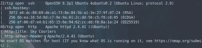


 The idea that established companies can miss out on the benefits of disruptive technologies because they cannot make the necessary changes to their existing business models.


 Info: A Poisson distribution is a type of probability distribution that helps to calculate the chance of a certain number of events happening in a given space or time period. It considers the average rate of these events and assumes they are independent of each other.
 At the point of writing, the EPL has gone halfway. It is now becoming more interesting than when it commenced. Arsenal’s dramatic resurgence means they are seen by many as favorites to win the crown. Manchester City are relentlessly in hot pursuit, especially with the arrival of Erling Haaland. Newcastle have become a surprising contender for the title.


 Story Recap: The Matrix Trilogy tells the story of Neo, a computer hacker who discovers that the world he knows is actually an elaborate virtual reality created by sentient machines. He joins a group of rebels led by Morpheus and Trinity, who have discovered the truth about the Matrix and are fighting to free humanity from its control. In order to save humanity, Neo must battle the machines and their agents, including the ruthless Agent Smith. Ultimately, Neo must make the ultimate sacrifice to save humanity from the machines.
 Reality Test: Harari provides a solid test to check if something is fiction or reality. Ask: can it suffer? The answer reveals whether “it” is real or a story. For example, money cannot suffer, so it must be a story or ideology. However, a human being or an animal can suffer so they must be real, according to the suffering test.
 ChatGPT: “The truth beyond the Matrix is the power of the individual. It’s the power to choose our own paths, to pursue our own dreams, and live life on our own terms. It’s the power to be true to ourselves, to be in control of our own destiny, and to be free from the confines of the system. It’s the freedom to be who we truly are, without fear or judgement, and to live life with purpose and joy.”


 Question: Given a Python string. How to encrypt the Python string using a password or otherwise and decrypt the encrypted phrase to obtain the initial cleartext again?


