Hot on the heels of the Blender 2.91 release, Blender 2.92 is currently in Alpha and one of the most exciting new features is Geometry Nodes. Part of the everything as nodes strategy for future Blender development, the addition of geometry nodes will add procedural capabilities to Blender without requiring programming or scripting. Before the 2.92 alpha, Geometry Nodes were a separate branch with the project page available here.

When using Geometry Nodes, you are can create or modify geometry in your Blender scene using the new Geometry Node Editor. The process is very similar to the current way Shaders and Cycles materials are constructed. The selection of nodes are documented in the manual, however most descriptions are pretty sparse at this point. If you want to get started with nodes you need to run Blender 2.92 or later. Until it is formally released, the best place to get alpha and beta Blender releases is here.

There are two example projects to get you started. The best one currently is this one which shows how to use nodes to scatter rocks across your scene. There is another project that will showcase how to procedurally create a tree, however this project is currently just a place holder.

You can learn more about Blender 2.92 and Geometry Nodes in the video below.

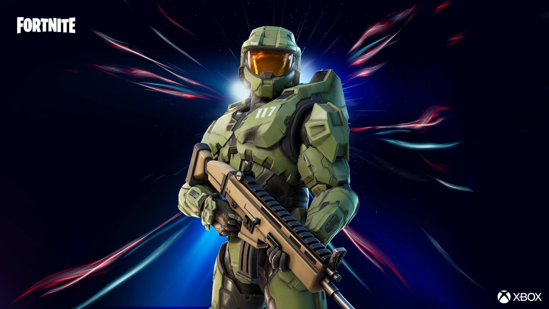
If you’ve ever wanted to play as Master Chief on the Switch, now you can…in the battle royale game Fortnite. At the 2020 Game Awards yesterday, the rumour about the protagonist of Xbox’s Halo series joining Epic’s insanely popular title came true.

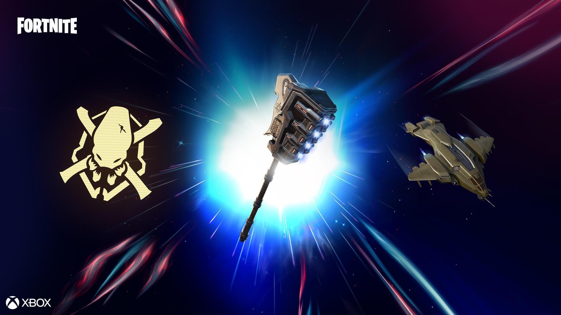
The Chief is available for 1500 V-Bucks, or you can get his entire set for 2600 V-Bucks. His pack comes with a UNSC Pelican Glider, a holographic Elite skull and a Gravity Hammer Pickaxe. In addition to this is a Lil’ Warthog emote.

To celebrate the addition of this new outfit, there’s also a recreation of the Halo multiplayer map Blood Gulch in Fortnite Creative. Here you can play a game of Capture the Flag. Find it in the ‘Featured Hub’ section of the game.

Master Chief follows on from the announcement of the God of War, Kratos. These characters are also being joined by Daryl Dixon and Michonne from The Walking Dead series. Will you be booting up Fortnite to see the Chief in action? Comment below.

2020 may have been a bumper year for video game sales, but it’s impacted other businesses in a very negative way. Cinemas and restaurants have been forced to close to prevent the spread of COVID-19, and while video game sales have been buoyant thanks digital and online purchases, physical retail stores with no means of selling remotely have seen their footfall reduced to a trickle; these bricks-and-mortar shops have really felt the pinch of local lockdowns and other restrictions on face-to-face trade.

You might think this is the worst possible time to open such a store, but that hasn’t stopped Richard Tewkesbury. You might recall him from a feature we did not so long ago; via his Game Boy Shack online store, he’s been selling games and modded systems for years, and his stall has been a regular face at live events throughout the UK – until 2020, of course.

With his income from events reduced to zero, Richard has taken it as an opportunity to fulfil a lifelong dream instead – to have his own physical retail store in his hometown of Leicester in the United Kingdom (which just so happens to be the closest city to Nintendo Life’s Loughborough HQ, fact fans).

If you’ve been following the coronavirus pandemic in the UK then you might be aware that Leicester was one of the first UK cities to be placed in lockdown earlier this year, and currently sits in “tier 3” – which is basically the highest of the three tiers laid out by the UK government. While this still allows for non-essential shops to remain open, the situation in the country – and indeed the entire world – still balances on a knife-edge and the UK has only just emerged from a ‘circuit breaker’ lockdown which could easily be repeated again in the near future. Nonetheless, Richard has opened his shop as planned, and has found that the reception has been an incredibly positive one.

Located close to the city’s main shopping complex, Super Game Shack (for that is its name) is described by its owner as something of a geek’s paradise; inside, you’ll find retro games and systems, Nintendo plushes, modded Game Boy consoles, video game-related merchandise and even Japanese sweets and drinks. Richard has stated that he wants to have a small workspace in the store so he can continue to create his trademark modded Game Boy consoles, and that in the fullness of time, retro fans will be able to visit to trade in old (and new) games for either cash or store credit, which will enable him to maintain a healthy turnover of pre-owned stock.

If you’re in the UK and based in Leicestershire (restrictions mean travelling between counties isn’t permitted) then be sure to drop by Super Game Shack and say hello to Rich (you can also follow the store via its Instagram and Facebook pages). He’s hopeful that the shop will be successful enough to become a truly permanent fixture in the city – and from what we’ve seen so far, it fully deserves to be.

Super Game Shack can be found at Unit 4, Silver Arcade, Leicester.

This article explores the use of the functions .UnivariateSpline() and .LSQUnivariateSpline(), from the Scipy package.

What Are Splines?

Splines are mathematical functions that describe an ensemble of polynomials which are interconnected with each other in specific points called the knots of the spline.

They’re used to interpolate a set of data points with a function that shows a continuity among the considered range; this also means that the splines will generate a smooth function, which avoid abrupt changes in slope.

Compared to the more classical fitting methods, the main advantage of splines is that the polynomial equation is not the same throughout the whole range of data points.

Instead, the fitting function can change from one interval to the subsequent one, allowing for fitting and interpolation of very complicated point distributions. In this article we will see:

• i) how to generate a spline function to fit a given set of data points,
• ii) which functions we can then use to extrapolate the value of points within the fitted range,
• iii) how to improve the fitting, and
• iv) how to calculate the related error.   

Splines — A Mathematical Perspective

In mathematics, splines are functions described by an ensemble of polynomials.

Even if splines seem to be described by a single equation, they are defined by different polynomial functions which holds over a specific range of points, whose extremes are called knots. Each knot hence represents a change in the polynomial function that is describing the shape of the spline in that specific interval.

One of the main characteristics of splines is their continuity; they are continuous along the entire interval in which they are defined; this allows for the generation of a smooth curve, that fit our set of data points.

One of the main advantages of using splines for fitting problems, instead of single polynomials, is the possibility of using lower degree polynomial functions to describe very complicated functions.

Indeed, if we wanted to use a single polynomial function, the degree of the polynomial usually increases with the complexity of the function that has to be described; increasing the degree of the fitting polynomial could introduce unwanted errors in the problem.

Here is a nice video that explain in simple terms this issue:

Splines avoid this by varying the fitting equation over the different intervals that characterize the initial set of data points. From an historical point of view, the word “Spline” comes from the flexible spline devices that were exploited by the shipbuilders to draw smooth shapes in the designing of vessels. Nowadays they also find large application as fundamental tools in lots of CAD software (https://en.wikipedia.org/wiki/Spline_(mathematics) ). 

Scipy.UnivariateSpline

In the first part of this article we explore the function .UnivariateSpline(); which can be used to fit a spline of a specific degree to some data points.

To understand how this function works, we start by generating our initial x and y arrays of data points. The x array (called “x”), is defined by using the np.linspace() function; the y array is defined by exploiting the np.random function called .randn(), which return a sample from the standard normal distribution.

See: https://numpy.org/devdocs/reference/random/generated/numpy.random.randn.html for additional documentation.

import matplotlib.pyplot as plt

from scipy.interpolate import UnivariateSpline, LSQUnivariateSpline

import numpy as np #x and y array definition (initial set of data points)

x = np.linspace(0, 10, 30)

y = np.sin(0.5*x)*np.sin(x*np.random.randn(30))

Once we have defined the initial set of data points, we can call the function .UnivariateSpline(), from the Scipy package and calculate the spline that best fits our points.

While the procedure is rather simple, understanding the fundamental parameters that define the spline function that we want to create, might generate some confusion; to this purpose, it is better to analyze in detail the main input parameters that can be defined when calling the function in our code.

As can be also seen in the documentation (https://docs.scipy.org/doc/scipy/reference/generated/scipy.interpolate.UnivariateSpline.html), the .UnivariateSpline() function accepts as mandatory inputs the x and y arrays of data points that we want to fit.

In most cases, our aim is to fit complicated functions and to this purpose, other parameters must be specified.

One of the most important parameters is “k”, which refers to the degree of the polynomials that define the spline segments. “k” can vary between one and five; increasing the degree of the polynomials allows a better fitting of more complicated functions; however, in order not to introduce artifacts in our fit; the best practice is to use the lower degree that allows for the better fitting procedure.

Another relevant parameter is “s”, it’s a float number which defines the so-called smoothing factor, which directly affects the number of knots present in the spline. More precisely, once we fix a specific value of “s”, the number of knots will be increased until the difference between the value of the original data points in the y array and their respective datapoints along the spline is less than the value of “s” (see documentation for the mathematical formula). It can be understood that the lower the value of “s”, the higher the fitting accuracy and (most of the times) the n° of knots, since we are asking for a smaller difference between the original points and the fitted ones.

Now that the parameters that governs the shape of our spline are clearer, we can return to the code and define the spline function. In particular, we will give as input arrays the “x” and “y” arrays previously defined; the value of the smoothing factor is initially set to five while the parameter “k” is left with the default value, which is three.

#spline definition spline = UnivariateSpline(x, y, s = 5) 

The output of the .UnivariateSpline() function is the function that fit the given set of data points. At this point, we can generate a denser x array, called “x_spline” and evaluate the respective values on the y axis using the spline function just defined; we then store them in the array “y_spline” and generate the plot.

x_spline = np.linspace(0, 10, 1000)

y_spline = spline(x_spline)

#Plotting

fig = plt.figure()

ax = fig.subplots()

ax.scatter(x, y)

ax.plot(x_spline, y_spline, 'g')

plt.show()

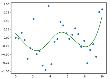
The result of this procedure is displayed in Figure 1.

As can be seen from Figure 1, the obtained spline gives a really bad fit of our initial data points; the main reason is the relatively high value that was assigned to the smoothing factor; we will now explore a possible strategy for improving our spline, without introducing exaggerated alterations.

One of the best way to improve this situation is to exploit the method .set_smoothing_factor(s); which continues the spline calculation according to a new smoothing factor (“s”, given as the only input), without altering the knots already found during the last call. This represents a convenient strategy, indeed, splines might be very sensitive to changes in the smoothing factor; this means that changing the smoothing function, directly in the .UnivariateSpline() calling, might alter significantly the output result in term of the spline shape (keep in mind that our goal is always to obtain the best fit with the simplest spline possible). The following code lines describe the definition of a new and more accurate spline function, with a smoothing factor equal to 0.5.

After the application of the above-mentioned method, the procedure is identical to the one described for generating the first spline.

# Changing the smoothing factor for a better fit

spline.set_smoothing_factor(0.05)

y_spline2 = spline(x_spline)

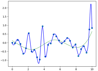
We conclude by plotting the result; Figure 2 display the final output, the new spline is the blue curve, plotted together with the old one (green curve) and the initial data points (light blue points).

#Plotting

fig = plt.figure()

ax = fig.subplots()

ax.scatter(x, y)

ax.plot(x_spline, y_spline, 'g', alpha =0.5)

ax.plot(x_spline, y_spline2, 'b')

plt.show()

As can be seen from Figure 2, the newly generated spline function well describes the initial data points and still pass by the knots that were found in the initial call (data points common to both the two spline functions)

We conclude this part by illustrating some useful methods that can be used after the generation of the correct spline function, for describing our data points. The first of these methods is called “.__call__(x)”, which allows evaluating the value of specific points on the spline, given in the form of a list or single number. The following lines describe the application of this methods (we evaluate the the spline for a value of 2 in the x-axis).

#evaluate point along the spline

print(spline.__call__(2))

The result of the print command is 0.5029480519149454. Another important method is .get_residual(), which allows obtaining the weighted sum of squared residuals of the spline approximation (more simply, an evaluation of the error in the fitting procedure).

#get the residuals

print(spline.get_residual())

The result for this case is 0.049997585478530546. In some applications, it could be of some interest to calculate the definite integral of the spline (i.e. the area underneath the spline curve between a specific range along the x-axis); to do this, the method .integral(a,b) represents the simplest solution; “a” and “b” are the lower and upper limits along the x-axis between which we want to evaluate the area (in this case we calculate the area underneath the spline, between 1 and 2). Application of this method is illustrated in the following lines.

#definite integral of the spline

print(spline.integral(1,2))

The result of the integration is -0.2935394976155577. The last method allows obtaining the values of the points in which the spline crosses the x-axis, i.e. the solutions to the equations defining the spline function. The method is called .roots(), its application is shown in the following lines.

#finding the roots of the spline function

print(spline.roots())

The output of this last line is an array containing the values of the points for which the spline crosses the x-axis, namely:

[1.21877130e-03 3.90089909e-01 9.40446113e-01 1.82311679e+00 2.26648393e+00 3.59588983e+00 3.99603385e+00 4.84430942e+00 6.04000192e+00 6.29857365e+00 7.33532448e+00 9.54966590e+00]

Scipy.LSQUnivariateSpline

In the last part of this article, we introduce .LSQUnivariateSpline(), another function that can be used for spline generation. From a practical point of view, it works similarly to .UnivariateSpline(), indeed as we will see, there are very few differences in how we call and define it in our script.

The fundamental difference between this function and the previous one, is that .LSQUnivariateSpline() allows generating spline curves by directly controlling the number and the position of the knots.

This means that we have the full control of the knots that will define the spline; differently, in the previous case, the number of knots was indirectly regulated through the choice of the smoothing factor. In order to appreciate how our spline will change by increasing the number of knots, we start by defining two different arrays, “t” and “t1”, t1 is the denser array.

#LSQUnivariateSpline

t = np.array([0.5, 1, 2.5])

t1 = np.linspace(1, 9, 20)

The function .LSQUnivariateSpline() accepts as mandatory input, the x, y arrays and the array “t”, which contains the coordinates of the knots that will define our spline. An important condition that has to be kept in mind is that the coordinates of the knots must be located within the range of the x array.

In our case, we will use the same x and y arrays employed for the previous case. At this point we have to call the function twice, in order to show the difference between the two set of knots arrays. In addition, we specify the parameter “k”, which again refers to the degree of the polynomials that describe the spline.

LSQUspline = LSQUnivariateSpline(x, y, t1, k = 4)

LSQUspline1 = LSQUnivariateSpline(x, y, t, k = 4)

Our final task is to plot the two splines, together with the original data points. We will generate the arrays containing the y values of the two splines directly in the plotting command.

#Plotting

plt.scatter(x, y, s=8)

plt.plot(x_spline, LSQUspline(x_spline), color = 'b')

plt.plot(x_spline, LSQUspline1(x_spline), color = 'g')

plt.show()

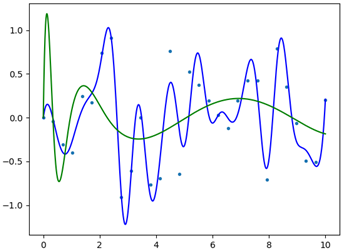
The final result is displayed in Figure 3; as can be seen, by increasing the number of knots, the spline function better approximates our data points. If we check carefully, both the splines pass for the knots specified in the “t” and “t1” arrays, respectively. Most of the methods previously shown for .UnivariateSpline() work on this function too (for additional documentation please refer to https://docs.scipy.org/doc/scipy/reference/generated/scipy.interpolate.LSQUnivariateSpline.html ).

Conclusion

To conclude, in this article, we explored spline functions, their power and versatility.

One thing that is important to keep in mind is that when we are using splines for fitting and interpolating a given set of data points, we should never exceeds with the degree of the polynomials that define the spline; this is to avoid unwanted errors and incorrect interpretation of the initial data.

The process has to be accurately refined, possibly through repetitive iterations to double check the validity of the generated output.

The post Fitting Data With Scipy’s UnivariateSpline() and LSQUnivariateSpline() first appeared on Finxter.

It basically pretends to be one of those old Infocom-style adventure games, but with no limits on what the player can enter. Whatever the input is, it improvises events through prose, to react to them.

While it’s still not up to the level of classic or modern text adventures, and occasionally loses track of situations over multiple turns, AI Dungeon 2 sometimes surprises in the kinds of responses it can generate, and the unexpected directions it can take the user’s adventures.

The game was created by Nick Walton of Brigham Young University’s Perception, Control, and Cognition Laboratory and created quite a stir upon its unveiling, so much that they had to quickly rework it to cut down on bandwidth costs. Walton answered some questions we had about how AI Dungeon 2 was made and where it’s going next.

Who are you, what is AI Dungeon 2, and who helped make it a reality?

I’ve been working on deep learning tech for the past couple years. I interned at a couple autonomous vehicle companies and have been doing research in the BYU Perception, Control, and Cognition Laboratory​, a deep learning research lab at BYU.

I’ve been working on AI Dungeon since I had the idea at a hackathon in March. I continued to work on the idea, getting advice from Dr. David Wingate, the professor I worked with. Eventually it finally came together as AI Dungeon 2 at the beginning of December.

AI Dungeon is a first of its kind game where the story and responses to your actions are entirely generated by deep learning. The awesome thing about this is the game is built on top of a giant machine learning model made by OpenAI called GPT-2 it can adapt and respond to almost any action you can imagine, giving you vast amounts of freedom that players have never had in a game before.

AI Dungeon 2‘s popularity shot up suddenly, almost overnight. What happened?

I had gotten some attention with AI Dungeon 1. A couple thousand people had played it when I had released it back in May, so when I started teasing snippets from AI Dungeon 2 people started paying attention. But when I actually released AI Dungeon 2 it exploded much faster than I had expected.

We had released it as a game people could play in Google Colab, a way for researchers to run code on Google machines for free, but it would download the 5 GB model each time someone played.

Within a few days we had racked up over $20,000 in bandwidth charges from so many people downloading the model. We had to temporarily shut it down until some awesome community contributors put up a peer to peer downloading solution.

Now AI Dungeon 2 is playable as a web and mobile app and a team has come together to work on improving the game. An awesome app developer Braydon Batungbacal built out the mobile apps in a week, my brother Alan Walton helped us build out the infrastructure to host the massive model at a large scale, and Thorsten Kreutz is helping us work on the long term of where this idea can go. We see AI Dungeon 2 as just the beginning of an exciting shift in entertainment.

Yeah there is a decent amount of model and data massaging that happens on the game side to make sure the model plays nicely. We cut off trailing sentences and end of text tokens in the model output as well as do some transforming on the player’s input to make sure it’s in the second person format. I also had to do a decent amount of work to control repetition as that’s a big problem with GPT-2 especially at lower temperature (randomness) settings.

It is a fun hobbyist programmer project to make your own text generator. GPT-2, while a great deal more sophisticated and using a much larger set of data, seems to do a similar kind of thing. Could you give us an overview of how it works?

GPT-2 is a deep learning language model. A language model essentially just means it tries to predict the most likely next word given the previous set of words. The really cool thing about language models is because you can train it on any text (no labeling required) it can learn from the really massive amount of text data that’s out there. The largest model was trained on 40 GB of just text data.

In learning to predict the most likely next word, it learns not just how the English language works, but it also learns a model of the world that allows it to predict the most likely next event (for example if you get stabbed you might die) and that allows you to use it to do some really interesting things.

The GPT-2 system is available for download for people who’d like to play around with it. How would you recommend interested people might get started?

The site for AI Dungeon 2 notes that you’re beginning to sell mobile app interfaces to help fund the server and bandwidth that the game requires. How is that going? Are you still worried that the project may have to end due to financial concerns?

We’ve turned the game into a startup as there’s really no way to make a great experience without having the financial sustainability of a business. We plan on keeping the base version of the game free to play, but will add a premium version of the game that will allow us to cover the server costs.

The premium version will have a lot of interesting new game modes and features so we’re pretty confident we’ll be able to make the game sustainable with that.

Is AI Dungeon 2, as it stands, complete? Are there any improvements, or a sequel, planned? Maybe allowing for more starting points, or to provide greater continuity between turns?

We have a lot of different things we’re working on. In the near term, we’re working on adding multiplayer and text to voice support, but we’re also looking at more innovative improvements in the future.

Text generation will continue to be a big part of what we’re trying to make with AI Dungeon and its sequels, but we’ll also start adding in other forms of AI content generation with music, images, and voice as we’re able to.

Most of our readers are game developers, and some of those use bespoke algorithms to do things like randomly generate terrain to explore. GPT-2 is built to generate text based on other text found on the internet; do you think the underlying system might someday be of use in the production of more traditional types of entertainment software?

Definitely. I think AI Dungeon is just the beginning in a huge evolution in gaming and we’re hoping to help enable that. There’s a lot of exciting potentials this technology opens up and we’re excited to see what that future looks like.

The UK games industry made a record £2.91 billion ($3.84 billion) contribution to the country’s national economy in 2019.

That’s according to new economic estimates released by the Department of Digital, Culture, Media, and Sport (DCMS), which reveals the industry contributed £2.91 billion ($3.84 billion) in gross value added (GVA) through development and publishing — representing a 9.1 percent increase on 2018.

Industry trade body Ukie has suggested the latest estimates show the UK video game sector will play pivotal role in helping the region’s economy recover from the coronavirus pandemic.

It also noted that the latest numbers only accord for the impact of game development and publishing, suggesting the “full size and economic contribution” of the entire UK games industry — including support services, retail, esports, and merchandising — could be even larger.

“These new figures underline how successfully, and quickly, the UK industry is growing. With leveling up firmly on the Government’s agenda, it makes perfect sense to back a sector that has 55 percent of game development roles based outside London,” commented Ukie CEO, Dr Jo Twist, in a blog post.

“That’s why we’re calling for greater and longer-term investment into the UK Games Fund and into an industry matched skills fund. The UK needs to show it can lead the world while backing local communities and the best way to do that is to back the modern, innovative and resilient games sector.”