
+- Sick Gaming (https://sickgaming.net)
+-- Forum: Programming (https://sickgaming.net/forum-76.html)
+--- Forum: Python (https://sickgaming.net/forum-83.html)
+--- Thread: [Tut] Matplotlib Scatter Plot – Simple Illustrated Guide (/thread-98443.html)
[Tut] Matplotlib Scatter Plot – Simple Illustrated Guide - xSicKxBot - 11-24-2020
Matplotlib Scatter Plot – Simple Illustrated Guide
Scatter plots are a key tool in any Data Analyst’s arsenal. If you want to see the relationship between two variables, you are usually going to make a scatter plot.
In this article, you’ll learn the basic and intermediate concepts to create stunning matplotlib scatter plots.
Matplotlib Scatter Plot Example
Let’s imagine you work in a restaurant. You get paid a small wage and so make most of your money through tips. You want to make as much money as possible and so want to maximize the amount of tips. In the last month, you waited 244 tables and collected data about them all.
We’re going to explore this data using scatter plots. We want to see if there are any relationships between the variables. If there are, we can use them to earn more in future.
- Note: this dataset comes built-in as part of the library.Code:
seaborn
First, let’s import the modules we’ll be using and load the dataset.
Code:
import matplotlib.pyplot as plt
import seaborn as sns # Optional step
# Seaborn's default settings look much nicer than matplotlib
sns.set() tips_df = sns.load_dataset('tips') total_bill = tips_df.total_bill.to_numpy()
tip = tips_df.tip.to_numpy()
The variable
Code:
tips_dfCode:
total_billLet’s make a scatter plot of
Code:
total_billCode:
plt.scatter()Code:
plt.scatter(total_bill, tip)
plt.show()
Nice! It looks like there is a positive correlation between a
Code:
total_billCode:
tipMatplotlib Scatter Plot with Labels
Labels are the text on the axes. They tell us more about the plot and is it essential you include them on every plot you make.
Let’s add some axis labels and a title to make our scatter plot easier to understand.
Code:
plt.scatter(total_bill, tip)
plt.title('Total Bill vs Tip')
plt.xlabel('Total Bill ($)')
plt.ylabel('Tip ($)')
plt.show()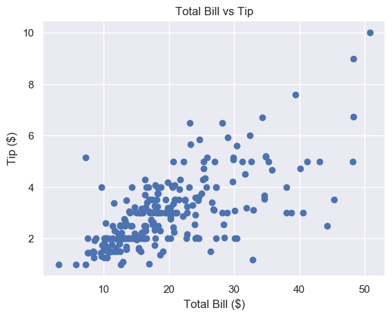
Much better. To save space, we won’t include the label or title code from now on, but make sure you do.
This looks nice but the markers are quite large. It’s hard to see the relationship in the $10-$30 total bill range.
We can fix this by changing the marker size.
Matplotlib Scatter Marker Size
The
Code:
sCode:
plt.scatter()Matplotlib Scatter Marker Size – Scalar
In
Code:
plt.scatter()Code:
s=72Thedocs define
Code:
sThe marker size in points**2.
This means that if we want a marker to have area 5, we must write
Code:
s=5**2The other matplotlib functions do not define marker size in this way. For most of them, if you want markers with area 5, you write
Code:
s=5Code:
plt.scatter()One way to remember this syntax is that graphs are made up of square regions. Markers color certain areas of those regions. To get the area of a square region, we do
Code:
length**2To set the best marker size for a scatter plot, draw it a few times with different
Code:
sCode:
# Small s
plt.scatter(total_bill, tip, s=1)
plt.show()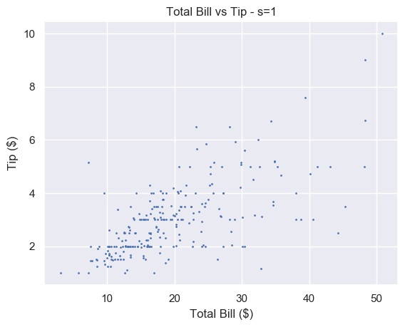
A small number makes each marker small. Setting
Code:
s=1Code:
sCode:
# Big s
plt.scatter(total_bill, tip, s=100)
plt.show()
Alternatively, a large number makes the markers bigger. This is too big for our plot and obscures a lot of the data.
We think that
Code:
s=20Code:
# Just right
plt.scatter(total_bill, tip, s=20)
plt.show()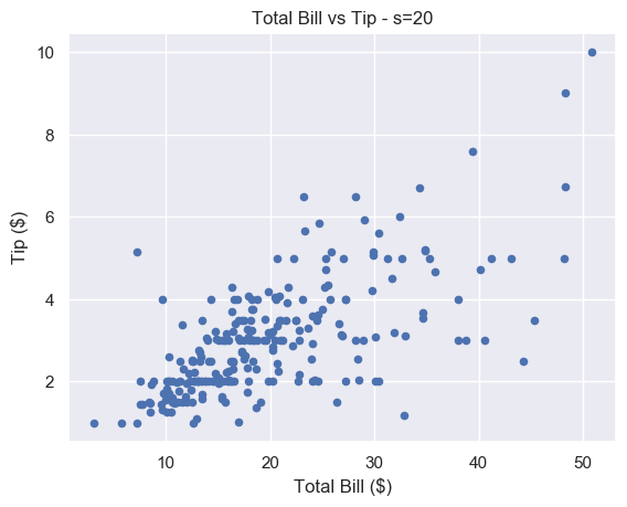
There is still some overlap between points but it is easier to spot. And unlike for
Code:
s=1Matplotlib Scatter Marker Size – Array
If we pass an array to
Code:
sYou also recorded the size of each of table you waited. This is stored in the NumPy array
Code:
size_of_tableCode:
# Select column 'size' and turn into a numpy array
size_of_table = tips_df['size'].to_numpy() # Increase marker size to make plot easier to read
size_of_table_scaled = [3*s**2 for s in size_of_table] plt.scatter(total_bill, tip, s=size_of_table_scaled)
plt.show()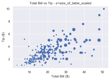
Not only does the tip increase when total bill increases, but serving more people leads to a bigger tip as well. This is in line with what we’d expect and it’s great our data fits our assumptions.
Why did we scale the
Code:
size_of_tableCode:
sCode:
s=1Code:
s=6
So we first square each value and multiply it by 3 to make the size difference more pronounced.
We should label everything on our graphs, so let’s add a legend.
Matplotlib Scatter Legend
To add a legend we use the
Code:
plt.legend()Code:
labelCode:
plt.legend()But we have a problem. We’ve only got one set of data here. We cannot label the points individually using the
Code:
labelHow do we solve this problem?
We could create 6 different datasets, plot them on top of each other and give each a different size and label. But this is time-consuming and not scalable.
Fortunately, matplotlib has a scatter plot method we can use. It’s called the
Code:
legend_elements()The elements in this scatter plot are different sizes. We have 6 different sized points to represent the 6 different sized tables. So we want
Code:
legend_elements()Let’s figure out how
Code:
legend_elements()Code:
# legend_elements() is a method so we must name our scatter plot
scatter = plt.scatter(total_bill, tip, s=size_of_table_scaled) legend = scatter.legend_elements() print(legend)
# ([], [])
Calling
Code:
legend_elements()Thedocs tell us
Code:
legend_elements()Code:
(handles, labels)Code:
plt.legend()The
Code:
plt.legend()Code:
plt.legend(handles, labels)Code:
scatter.legend_elements()Code:
*Code:
# Method 1 - unpack tuple using *
legend = scatter.legend_elements()
plt.legend(*legend) # Method 2 - unpack tuple into 2 variables
handles, labels = scatter.legend_elements()
plt.legend(handles, labels)
Both produce the same result. The matplotlib docs use method 1. Yet method 2 gives us more flexibility. If we don’t like the labels matplotlib creates, we can overwrite them ourselves (as we will see in a moment).
Currently,
Code:
handlesCode:
labelsCode:
legend_elements()There are4 optional arguments but let’s focus on the most important one:
Code:
propCode:
PropCode:
'colors'Code:
'sizes'We will look at different colored scatter plots in the next section. As our plot contains 6 different sized markers, we set
Code:
prop='sizes'Code:
scatter = plt.scatter(total_bill, tip, s=size_of_table_scaled) handles, labels = scatter.legend_elements(prop='sizes')Now let’s look at the contents of
Code:
handlesCode:
labelsCode:
>>> type(handles)
list
>>> len(handles)
6 >>> handles
[<matplotlib.lines.Line2D object at 0x1a2336c650>,
<matplotlib.lines.Line2D object at 0x1a2336bd90>,
<matplotlib.lines.Line2D object at 0x1a2336cbd0>,
<matplotlib.lines.Line2D object at 0x1a2336cc90>,
<matplotlib.lines.Line2D object at 0x1a2336ce50>,
<matplotlib.lines.Line2D object at 0x1a230e1150>]
Handles is a list of length 6. Each element in the list is a
Code:
matplotlib.lines.Line2DCode:
plt.legend()Code:
'picture'It is possible tocreate custom handles but this is out of the scope of this article. Now let’s look at
Code:
labelsCode:
>>> type(labels)
list
>>> len(labels)
6 >>> labels
['$\\mathdefault{3}$', '$\\mathdefault{12}$', '$\\mathdefault{27}$', '$\\mathdefault{48}$', '$\\mathdefault{75}$', '$\\mathdefault{108}$']
Again, we have a list of length 6. Each element is a string. Each string is written using LaTeX notation
Code:
'$...$'Why these numbers? Because they are the unique values in the list
Code:
size_of_table_scaledCode:
>>> np.unique(size_of_table_scaled)
array([ 3, 12, 27, 48, 75, 108])
We used these numbers because using 1-6 is not enough of a size difference for humans to notice.
However, for our legend, we want to use the numbers 1-6 as this is the actual table size. So let’s overwrite
Code:
labelsCode:
labels = ['1', '2', '3', '4', '5', '6']Note that each element must be a string.
We now have everything we need to create a legend. Let’s put this together.
Code:
# Increase marker size to make plot easier to read
size_of_table_scaled = [3*s**2 for s in size_of_table] # Scatter plot with marker sizes proportional to table size
scatter = plt.scatter(total_bill, tip, s=size_of_table_scaled) # Generate handles and labels using legend_elements method
handles, labels = scatter.legend_elements(prop='sizes') # Overwrite labels with the numbers 1-6 as strings
labels = ['1', '2', '3', '4', '5', '6'] # Add a title to legend with title keyword
plt.legend(handles, labels, title='Table Size')
plt.show()
Perfect, we have a legend that shows the reader exactly what the graph represents. It is easy to understand and adds a lot of value to the plot.
Now let’s look at another way to represent multiple variables on our scatter plot: color.
Matplotlib Scatter Plot Color
Color is an incredibly important part of plotting. It could be an entire article in itself. Check out the Seaborndocs for a great overview.
Color can make or break your plot. Some color schemes make it ridiculously easy to understand the data. Others make it impossible.
However, one reason to change the color is purely for aesthetics.
We choose the color of points in
Code:
plt.scatter()Code:
cCode:
colorYou can set any color you want using an RGB or RGBA tuple (red, green, blue, alpha). Each element of these tuples is a float in
Code:
[0.0, 1.0]Code:
'#1f1f1f'- orCode:
'b'Code:'blue'
- orCode:
'r'Code:'red'
- orCode:
'g'Code:'green'
- orCode:
'k'Code:'black'
- orCode:
'w'Code:'white'
Here’s the plot of
Code:
total_billCode:
tip
For each plot, call
Code:
plt.scatter()Code:
total_billCode:
colorCode:
cCode:
# Blue (the default value)
plt.scatter(total_bill, tip, color='b') # Red
plt.scatter(total_bill, tip, color='r') # Green
plt.scatter(total_bill, tip, c='g') # Black
plt.scatter(total_bill, tip, c='k')Note: we put the plots on one figure to save space. We’ll cover how to do this in another article (hint: use
Code:
plt.subplots()Matplotlib Scatter Plot Different Colors
Our restaurant has a smoking area. We want to see if a group sitting in the smoking area affects the amount they tip.
We could show this by changing the size of the markers like above. But it doesn’t make much sense to do so. A bigger group logically implies a bigger marker. But marker size and being a smoker don’t have any connection and may be confusing for the reader.
Instead, we will color our markers differently to represent smokers and non-smokers.
We have split our data into four NumPy arrays:
- x-axis – non_smoking_total_bill, smoking_total_bill
- y-axis – non_smoking_tip, smoking_tip
If you draw multiple scatter plots at once, matplotlib colors them differently. This makes it easy to recognize the different datasets.

Code:
plt.scatter(non_smoking_total_bill, non_smoking_tip)
plt.scatter(smoking_total_bill, smoking_tip)
plt.show()
This looks great. It’s very easy to tell the orange and blue markers apart. The only problem is that we don’t know which is which. Let’s add a legend.
As we have 2
Code:
plt.scatter()Code:
plt.legend()Code:
# Add label names to each scatter plot
plt.scatter(non_smoking_total_bill, non_smoking_tip, label='Non-smoking')
plt.scatter(smoking_total_bill, smoking_tip, label='Smoking') # Put legend in upper left corner of the plot
plt.legend(loc='upper left')
plt.show()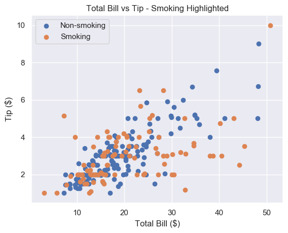
Much better. It seems that the smoker’s data is more spread out and flat than non-smoking data. This implies that smokers tip about the same regardless of their bill size. Let’s try to serve less smoking tables and more non-smoking ones.
This method works fine if we have separate data. But most of the time we don’t and separating it can be tedious.
Thankfully, like with
Code:
sizeCode:
cLet’s say we have a list
Code:
smokerCode:
plt.scatter(total_bill, tip, c=smoker)
plt.show()Note: if we pass an array/sequence, we must the keyword
Code:
cCode:
colorCode:
ValueErrorCode:
ValueError: 'color' kwarg must be an mpl color spec or sequence of color specs.
For a sequence of values to be color-mapped, use the 'c' argument instead.
Great, now we have a plot with two different colors in 2 lines of code. But the colors are hard to see.
Matplotlib Scatter Colormap
A colormap is a range of colors matplotlib uses to shade your plots. We set a colormap with the
Code:
cmapWe’ll choose
Code:
'bwr'If color theory interests you, we highly recommend thispaper. In it, the author creates
Code:
bwrCode:
plt.scatter(total_bill, tip, c=smoker, cmap='bwr')
plt.show()
Much better. Now let’s add a legend.
As we have one
Code:
plt.scatter()Code:
scatter.legend_elements()Code:
prop='colors'Code:
legend_elements()Code:
# legend_elements() is a method so we must name our scatter plot
scatter = plt.scatter(total_bill, tip, c=smoker_num, cmap='bwr') # No arguments necessary, default is prop='colors'
handles, labels = scatter.legend_elements() # Print out labels to see which appears first
print(labels)
# ['$\\mathdefault{0}$', '$\\mathdefault{1}$']
We unpack our legend into
Code:
handlesCode:
labelsNow we overwrite
Code:
labelsCode:
plt.legend()Code:
# Re-name labels to something easier to understand
labels = ['Non-Smokers', 'Smokers'] plt.legend(handles, labels)
plt.show()
This is a great scatter plot. It’s easy to distinguish between the colors and the legend tells us what they mean. As smoking is unhealthy, it’s also nice that this is represented by red as it suggests
Code:
'danger'What if we wanted to swap the colors?
Do the same as above but make the
Code:
smokerCode:
smokers_swapped = [1 - x for x in smokers]Finally, as 0 comes first, we overwrite
Code:
labelsCode:
labels = ['Smokers', 'Non-Smokers']
Matplotlib Scatter Marker Types
Instead of using color to represent smokers and non-smokers, we could use different marker types.
There are over 30built-in markers to choose from. Plus you can use any LaTeX expressions and even define your own shapes. We’ll cover the most common built-in types you’ll see. Thankfully, the syntax for choosing them is intuitive.
In our
Code:
plt.scatter()Code:
markerHere are the most common examples:
- – circle (default)Code:
'o'
- – triangle downCode:
'v'
- – triangle upCode:
'^'
- – squareCode:
's'
- – plusCode:
'+'
- – diamondCode:
'D'
- – thin diamondCode:
'd'
- – LaTeX syntax e.g.Code:
'$...$'makes each marker the Greek letter π.Code:'$\pi$'
Let’s see some examples

For each plot, call
Code:
plt.scatter()Code:
total_billCode:
markerCode:
# Circle
plt.scatter(total_bill, tip, marker='o') # Plus
plt.scatter(total_bill, tip, marker='+') # Diamond
plt.scatter(total_bill, tip, marker='D') # Triangle Up
plt.scatter(total_bill, tip, marker='^')
At the time of writing, you cannot pass an array to
Code:
markerCode:
colorCode:
sizeCode:
# Square marker
plt.scatter(non_smoking_total_bill, non_smoking_tip, marker='s', label='Non-smoking') # Plus marker
plt.scatter(smoking_total_bill, smoking_tip, marker='+', label='Smoking') plt.legend(loc='upper left')
plt.show()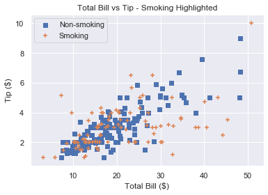
Remember that if you draw multiple scatter plots at once, matplotlib colors them differently. This makes it easy to recognise the different datasets. So there is little value in also changing the marker type.
To get a plot in one color with different marker types, set the same color for each plot and change each marker.
Code:
# Square marker, blue color
plt.scatter(non_smoking_total_bill, non_smoking_tip, marker='s', c='b' label='Non-smoking') # Plus marker, blue color
plt.scatter(smoking_total_bill, smoking_tip, marker='+', c='b' label='Smoking') plt.legend(loc='upper left')
plt.show()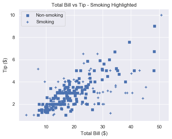
Most would agree that different colors are easier to distinguish than different markers. But now you have the ability to choose.
Summary
You now know the 4 most important things to make excellent scatter plots.
You can make basic matplotlib scatter plots. You can change the marker size to make the data easier to understand. And you can change the marker size based on another variable.
You’ve learned how to choose any color imaginable for your plot. Plus you can change the color based on another variable.
To add personality to your plots, you can use a custom marker type.
Finally, you can do all of this with an accompanying legend (something most Pythonistas don’t know how to use!).
Where To Go From Here
Do you want to earn more money? Are you in a dead-end 9-5 job? Do you dream of breaking free and coding full-time but aren’t sure how to get started?
Becoming a full-time coder is scary. There is so much coding info out there that it’s overwhelming.
Most tutorials teach you Python and tell you to get a full-time job.
That’s ok but why would you want another office job?
Don’t you crave freedom? Don’t you want to travel the world? Don’t you want to spend more time with your friends and family?
There are hardly any tutorials that teach you Python and how to be your own boss. And there are none that teach you how to make six figures a year.
Until now.
We are full-time Python freelancers. We work from anywhere in the world. We set our own schedules and hourly rates. Our calendars are booked out months in advance and we have a constant flow of new clients.
Sounds too good to be true, right?
Not at all. We want to show you the exact steps we used to get here. We want to give you a life of freedom. We want you to be a six-figure coder.
Click the link below to watch our pure-value webinar. We show you the exact steps to take you from where you are to a full-time Python freelancer. These are proven, no-BS methods that get you results fast.
https://tinyurl.com/python-freelancer-webinar
It doesn’t matter if you’re a Python novice or Python pro. If you are not making six figures/year with Python right now, you will learn something from this webinar.
Click the link below now and learn how to become a Python freelancer.
https://tinyurl.com/python-freelancer-webinar
References
- https://stackoverflow.com/questions/14827650/pyplot-scatter-plot-marker-size
- https://matplotlib.org/3.1.1/api/_as_gen/matplotlib.pyplot.scatter.html
- https://seaborn.pydata.org/generated/seaborn.scatterplot.html
- https://matplotlib.org/3.1.1/api/collections_api.html#matplotlib.collections.PathCollection.legend_elements
- https://blog.finxter.com/what-is-asterisk-in-python/
- https://matplotlib.org/3.1.1/api/markers_api.html#module-matplotlib.markers
- https://stackoverflow.com/questions/31726643/how-do-i-get-multiple-subplots-in-matplotlib
- https://matplotlib.org/3.1.0/gallery/color/named_colors.html
- https://matplotlib.org/3.1.0/tutorials/colors/colors.html#xkcd-colors
- https://github.com/matplotlib/matplotlib/issues/11155
- https://matplotlib.org/3.1.1/tutorials/colors/colormaps.html
- https://matplotlib.org/3.1.1/api/_as_gen/matplotlib.pyplot.legend.html
- https://matplotlib.org/tutorials/intermediate/legend_guide.html
- https://seaborn.pydata.org/tutorial/color_palettes.html
- https://cfwebprod.sandia.gov/cfdocs/CompResearch/docs/ColorMapsExpanded.pdf
- https://matplotlib.org/3.1.1/api/_as_gen/matplotlib.pyplot.subplots.html
The post Matplotlib Scatter Plot – Simple Illustrated Guide first appeared on Finxter.